Overview

This set of notes is intended to help introduce regression splines - terms intended to model non-linear effects in regression equations. I start by introducing polynomial terms which should be more familiar. Then I show how splines are similar, but tend behave better in many situations.

Making non-linear functions using polynomials

First we will start out with a simple set of data - violent crime rates in New York City from 1985 through 2010. Here is a table of that data, and below that is a scatterplot showing the relationship between the year and the violent crime rate per 100,000 population.

Year    Violent Crime Rate 
1985    1881.3
1986    1995.2
1987    2036.1
1988    2217.6
1989    2299.9
1990    2383.6
1991    2318.2
1992    2163.7
1993    2089.8
1994    1860.9
1995    1557.8
1996    1344.2
1997    1268.4
1998    1167.4
1999    1062.6
2000     945.2
2001     927.5
2002     789.6
2003     734.1
2004     687.4
2005     673.1
2006     637.9
2007     613.8
2008     580.3
2009     551.8
2010     593.1

You can see via the scatterplot that if we want to model the rate as some function of year, that it needs to be a non-linear function. Although one would typically consider time-series models for this problem (such as auto-regressive or moving average terms) ignore those options for now. This curve would be very similar if you say had a sample of individuals with ages from 16 through 40, and on the Y axis you had the percentage of individuals that committed a crime.

One simple way to model this as a non-linear relationship is to introduce polynomial terms, such as Year^2, Year^3, etc. Here the equation would subsequently be:

\[\text{Violent Crime Rate} = \beta_0 + \beta_1(\text{Year}) + \beta_2(\text{Year}^2) + \beta_3(\text{Year}^3) + \epsilon\]

To estimate this equation, I have to actually add the polynomial variables into my data set. So here I add in those terms, but first I subtract 1985 from the Years before doing so. Note that 2000^3 equals 8 billion - statistical software typically does not like so high of values. This subtraction does not make any material difference to the estimated terms though, in the end it just changes \(\beta_0\) - the intercept term. The predictions are the same. A common way to do this with yearly data is to have the years start at 0 or 1 (for say age). Another though for data is to subtract the mean of the data.

So our dataset now looks like:

Year       VCR  Y0  Y^2   Y^3
1985    1881.3   0    0     0
1986    1995.2   1    1     1
1987    2036.1   2    4     8
1988    2217.6   3    9    27
1989    2299.9   4   16    64
1990    2383.6   5   25   125
1991    2318.2   6   36   216
1992    2163.7   7   49   343
1993    2089.8   8   64   512
1994    1860.9   9   81   729
1995    1557.8  10  100  1000
1996    1344.2  11  121  1331
1997    1268.4  12  144  1728
1998    1167.4  13  169  2197
1999    1062.6  14  196  2744
2000     945.2  15  225  3375
2001     927.5  16  256  4096
2002     789.6  17  289  4913
2003     734.1  18  324  5832
2004     687.4  19  361  6859
2005     673.1  20  400  8000
2006     637.9  21  441  9261
2007     613.8  22  484 10648
2008     580.3  23  529 12167
2009     551.8  24  576 13824
2010     593.1  25  625 15625

So fitting this equation we end up with the results below (rounded to the nearest integer).

\[\text{Violent Crime Rate} = 1943 + 149(\text{Year}) + -23(\text{Year}^2) + 1(\text{Year}^3) + \epsilon\]

Below I plotted the predictions from this equation as a red line.

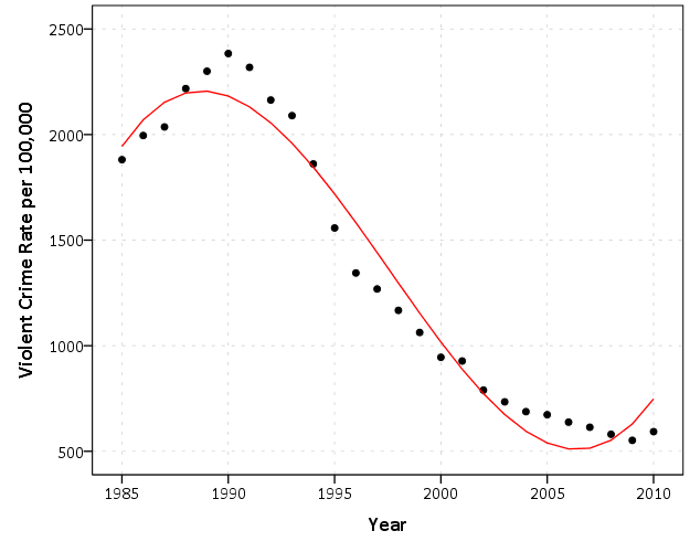
You can see that is not a great fit. In general with regression it won’t hit the peak (it will be regressed more towards the mean), but you would still want the apex of the line to be close to the actual apex in the data. Here the cubic line peaks a few years to early. Also a problem with polynomials is the tails. You can see it pits around 2007 and then begins to climb back up. So forecasting outside of the data would be disastrous - but that is the nature of polynomial terms - it has to have those two bends. Those bends though influence the path of the entire function though.

Using Splines instead of Polynomials

So instead of using polynomial terms, I suggest to use regression splines in most situations. The formulas for regression splines are more complicated than polynomial terms, but they work the same way. You create a new set of variables (called basis functions), and then enter them on the right hand side of the regression equation.

So here is that complicated formula specifically for restricted cubic splines, but to note you do not need to memorize this, just know it is there. So we need two things, our original variable \(x\), and a set of \(K\) knot locations. The specific knot locations I will use lowercase \(k_i\) to note where they are. So \(k_1\) would be the location of the first knot, \(k_2\) would be the location of the second knot. Also \(k_K\) is the last knot, and \(k_{K-1}\) is the next to last knot location. With restricted cubic splines, you get out K-2 new variables - so you at least need to specify 3 knots. So if you have 5 knots you get 3 new variables.

So first we specify a set of indicator variables:

\[ \begin{matrix} u_+ = u \text{ if } u > 0 \\ u_+ = 0 \text{ if } u \leq 0 \end{matrix} \]

To explain this I need to introduce the full formula for a particular spline variable. So here is that full formula.

\[x_i = \Bigg[ (x - k_i)^3_+ \Bigg] - \Bigg[(x - k_{K-1})^3_+ \cdot \frac{k_K - k_i}{k_K - k_{K-1}}\Bigg] + \Bigg[(x - k_K)^3_+ \cdot \frac{k_{K-1} - k_i}{k_K - k_{K-1}}\Bigg]\]

Here \(x\) is the original variable you put in, and \(x_i\) is the spline transformed variable you get out. I’ve split the equation into three parts using the big square brackets. The first part is \(\Bigg[ (x - k_i)^3_+ \Bigg]\). Here what this means is that you take the original \(x\) value, subtract the \(k_i\) knot location, and cube that value. The final \(+\) subscript refers back to the indicator variable notation with the u’s I mentioned earlier. This means that if what is in the parentheses is zero, then set this number to zero.

To go through the motions of calculating this, for our original data lets say that our knot locations will be at the years 1989, 1993, 1998, and 2007. To make the cube terms simpler, we are going to be working with the Years - 1985 (so the first year in the sample starts at 0, 1986 = 1, etc.). So this means our four knot locations are at 3, 7, 12, and 21. So lets just fix our year we will be examining at 16 (2001), and see how that would be transformed by the restricted cubic spline regression.

So the first bracket we have \(\Bigg[ (x - k_i)^3_+ \Bigg]\). So our value of \(x\) is 16, and our value of \(k_i\) we will be considering the first knot, 3. So this equation is simply (16 - 3)^3, which equals 2197. If the year we were considering was less than 3, we would set this value to zero, per the indicator u notation (see the + subscript at the end of the parentheses).

The second bracket we introduce two new terms, \(k_K\) and \(k_{K-1}\) these are the last knot and the second to last knot location, which equal 21 and 12 respectively in our example. So this bracket then ends up being [(16 - 12)^3]*[(21 - 3)/(21 - 12)], which equals 128. Note again the plus notation after the first term in the parentheses in the formula before the fraction.

Finally we have the last bracket, \(\Bigg[(x - k_K)^3_+ \cdot \frac{k_{K-1} - k_i}{k_K - k_{K-1}}\Bigg]\). This was is easy, because \(x - k_K\) is not greater than 0 in our example, this whole term is equal to zero. So then to make our final value, note that it is the first bracket minus the second bracket plus the third bracket. So we have 2197 - 128 = 2069 is our transformed \(x_i\) value. Typically software again divides this number, to make sure the values are not too large. In the R and SPSS code I provide for class the end value is divided by \((k_K - k_1)^2\), which is (21-3)^2 = 324, so our final \(x_i\) value is then \(2069/324 \approx 6.4\).

In this example you would then go through the same motions, but instead of using the first knot location 3, you would use the second knot location, 7. You do not do the formulas for the last two knot locations, hence if you have \(K\) knots you then end up with \(K-2\) new basis variables. So with our sample data and four knots, doing this same exercise results in the below dataset, where S1 and S2 our are new variables.

Year       VCR  Y0    S1     S2  
1985    1881.3   0    .0     .0
1986    1995.2   1    .0     .0
1987    2036.1   2    .0     .0
1988    2217.6   3    .0     .0
1989    2299.9   4    .0     .0
1990    2383.6   5    .0     .0
1991    2318.2   6    .1     .0
1992    2163.7   7    .2     .0
1993    2089.8   8    .4     .0
1994    1860.9   9    .7     .0
1995    1557.8  10   1.1     .1
1996    1344.2  11   1.6     .2
1997    1268.4  12   2.3     .4
1998    1167.4  13   3.1     .7
1999    1062.6  14   4.1    1.0
2000     945.2  15   5.2    1.5
2001     927.5  16   6.4    1.9
2002     789.6  17   7.7    2.5
2003     734.1  18   9.1    3.1
2004     687.4  19  10.5    3.7
2005     673.1  20  12.0    4.3
2006     637.9  21  13.5    5.0
2007     613.8  22  15.0    5.6
2008     580.3  23  16.5    6.3
2009     551.8  24  18.1    7.0
2010     593.1  25  19.7    7.8

Here is our regression equation now with those spline variables:

\[\text{Violent Crime Rate} = \beta_0 + \beta_1(\text{Year}) + \beta_2(S_1) + \beta_3(S_2) + \epsilon\]

If you have many spline variables, I tend to like writing the equation as:

\[\text{Violent Crime Rate} = \beta_0 + g(S_k) + \epsilon\]

And then explain in text that \(g(S_k)\) refers to a function of the spline constructed variables.

And we can go ahead and fit our regression equation with these new variables. Here are the resulting coefficients for these variables. Note that we still include the original year term in the equation.

\[\text{Violent Crime Rate} = 1973 + 57(\text{Year}) + -944(S_1) + 2048(S_2) + \epsilon\]

And here is our predicted values for our spline locations.

You can see that the spline ended up fitting much better to this dataset than the polynomial function did using the same number of terms. Technically you could get a better and better fit by adding in more polynomial terms (e.g. Year^4, Year^5), but spline terms tend to be much more economical and fairly robust to where you place the knot locations. You still end up with a blip up at the end in this example, but the curve fits the data much more closely along the entire line.

Further literature

For further general references on regression splines, I would suggest examining Durrleman and Simon (1989) and Harrell Jr (2015). For an application of using splines to model the age-crime curve, you can see Liu (2015).

For the examples used in class, the non-linear terms for area, that is directly from my dissertation, one article is currently published in Wheeler (2017). That also includes interactions between spline terms to account for spatial trends, which are typically referred to as tensor splines.

In these examples you explicitly choose the knot locations for splines. One way to automatically choose the spline locations though is to start with many knots and then use a selection criteria to eliminate some (Marsh and Cormier 2001). This technique was used in Messner et al. (2005) to find when cities experienced crack related homicide booms. I don’t suggest this technique though, as you generally should not use model selection criteria and inference in one go.

A more efficient way to automatically select knot terms are to use shrinkage or cross-validation. These are the techniques used in the R package mgcv, written by Simon Wood. He has many articles on the topic, and so I would recommend his book, Wood (2017), if you are interested in identifying a non-linear function in a really automated fashion. Still I typically recommend just setting the knot locations at regular intervals along your independent variable.

References