Introduction

These are lecture notes on Poisson regression. It goes through how to interpret the Poisson distribution, fitting Poisson regression, and choosing whether you should use Negative Binomial instead of Poisson regression through some simple statistics. For a general book reference I would recommend Long (1997), but hopefully this is enough to get you started.

The Poisson Distribution

The Poisson distribution was originally formulated to describe the number of events that occur in a particular time period. Poisson was a French mathematician - not a fish. Many French mathematicians took as motivation criminal justice proceedings (see also Guerry or Quetelet), and this is true for Poisson as well. The Wikipedia page on the Poisson distribution lists he estimates the number of false convictions per country using the distribution.

So a few things to note about the Poisson distribution. It only has support on zero and all positive integers. This means the Poisson distribution could never predict a non-integer value, such as 2.5. It also means it will never predict a negative value, such as -3. Finally, it means that 0 needs to be a valid potential outcome, and there is no upper limit. If you have data that a zero cannot occur, say a dataset of the number of arrests individuals have, and they only show up if arrested (so there are not people with zero arrests in the dataset) then that is not Poisson distributed (but is a truncated Poisson distribution, see some of the notes at the end for using this information to estimate the number of zero's using capture-recapture models). If you have a dataset of delinquency items, and the number of items cannot go above the total number of questions (e.g. you ask 8 questions about delinquency and add them up, so values can only be integers from 0 to 8), then you have a binomial distribution (not to be later confused with the negative binomial distribution). See Britt, Rocque, and Zimmerman (2017) for example discussion of the delinquency items, and see (Andrew P Wheeler and Kovandzic 2017) for an example of modeling homicide rates using binomial models.¹

Real life data pretty much never perfectly conforms to theoretical distributions. For Poisson data, the inter-arrival times of events should be random. One way with crime data this is clearly violated is that crimes are sometimes reciprocal - one gang shooting may prompts a retaliation gang shooting. Another is that one offender may commit a spree of crimes in a short time period. Either of these will make the data not Poisson distribution, but overdispersed. I will take a bit more about that though when I bring up the negative binomial distribution.

For a few mathematical notes on the Poisson distribution. We often refer to the mean of the Poisson distribution using the Greek letter lambda, \(\lambda\). The Poisson has a special property that its variance equals its mean. So if you know the mean, you know all there is to know about how a Poisson distribution behaves. Since the Poisson distribution only has support on integer values, we describe it as having a probability mass function, instead of a probability density function (a PMF instead of a PDF). That probability mass function can be written as below, where \(\lambda\) is the mean of the distribution, and \(k\) is the particular integer value we are examining.

\[\frac{\lambda^k e^{-\lambda}}{k!}\]

So say we have a Poisson distribution with a mean of 2 (i.e. \(\lambda = 2\)), and we want to know the probability mass at the integer value of 1. This is how you would calculate it.

\[ \frac{\lambda^k e^{-\lambda}}{k!} = \frac{2^1 e^{-2}}{1!} \approx 0.27\]

What this means in plain English is that if we have a large sample (say the number of crimes per day over a year), if it is Poisson distributed we would expect about 27% of the days to have 1 crime. Doing the same for zero we would expect it to have under 14% zeroes. If you do this for all integer values, from 0 to some really high integer, you will eventually reach 100%.

Understanding this is important, as we will later on assess the fit of a Poisson regression equation by performing this operation on the predicted values. If say your model only predicts that 30% of the sample should have zero, and in reality you have 60%, you then need to use a different model. Probably a negative binomial regression model, which is very similar to the Poisson and I will go over in a following section.

Park and Eck (2013) also have several useful formula to understand how much random repeat victimization you would expect by chance due to the Poisson distribution.

Poisson Regression

Poisson regression is popular to predict crime counts for macro level data. A canonical citation in our field is Osgood (2000). The equation for Poisson regression can be written as (in the case of one independent variable \(X\)):

\[\log ( \mathbb{E}[Y] )= \beta_0 + \beta_1X \]

Note that one often swaps out lambda for the expectation of the outcome variable, e.g. \(\lambda = \mathbb{E}[Y]\). Writing it in terms of expected values shows its relationship to other generalized linear models though.

So lets go through a simple example. I will be using the data from my dissertation I have disseminated in class. If you are following along from elsewhere you can download data from my dissertation here.

So first I will be fitting a simple Poisson model predicting the number of Part 1 crimes on street units (either street midpoints or intersections) during one year as a function of the number of alcohol outlets on those street units (this includes both on-premise bars, as well as off-premise locations that can sell alcohol, like liquor stores or convenience stores that sell beer). So we fit a Poisson regression equation:

\[\log ( \mathbb{E}[\text{Crime}] )= \beta_0 + \beta_1\cdot(\text{Alcohol Lic.}) \]

And for this equation I subsequently get:

\[\log ( \mathbb{E}[\text{Crime}] )= 0.37 + 0.27\cdot(\text{Alcohol Lic.}) \]

Interpreting these coefficients are more tricky than with OLS models. So if you say wanted to compare a street with 0 alcohol outlets to a street with one outlet, you would have:

\[ \begin{matrix} \exp (0.37 + 0.27\cdot 0 ) \approx 1.4 \\ \exp (0.37 + 0.27\cdot 1 ) \approx 1.9 \end{matrix} \]

So that adding one alcohol outlet increases the number of Part 1 crimes on the street by about 0.5 crimes. This is more complicated though if you include additional independent variables in the equation. Say we also included the number of 311 calls for service on the street as a control variable, and we get an equation that is:

\[\log ( \mathbb{E}[\text{Crime}] )= 0.15 + 0.25\cdot(\text{Alcohol Lic.}) + 0.03\cdot(\text{311 Calls})\]

So now what happens if we want to predict the number of crimes adding one alcohol outlet increases crimes?

\[ \begin{matrix} \exp (0.15 + 0.25\cdot 0 + 0.03\cdot\text{311 Calls} ) = ? \\ \exp (0.15 + 0.25\cdot 1 + 0.03\cdot\text{311 Calls} ) = ? \end{matrix} \]

We have an unknown in the equation that will affect the outcome - we need to fill in some value for calls for service. To make reasonable predictions, you have to set the number of calls for service to some reasonable value. Here the mean number of 311 calls for service in the same is just over 5, so I will set it to 5 and see what happens to our predictions for adding one alcohol outlet on the street unit.

\[ \begin{matrix} \exp (0.15 + 0.25\cdot 0 + 0.03\cdot 5 ) \approx 1.3 \\ \exp (0.15 + 0.25\cdot 1 + 0.03\cdot 5 ) \approx 1.7 \end{matrix} \]

If we fill in a higher value you will see larger predictions and subsequently larger differences. Say we include 40 calls for service instead of 5.

\[ \begin{matrix} \exp (0.15 + 0.25\cdot 0 + 0.03\cdot 40 ) \approx 3.9 \\ \exp (0.15 + 0.25\cdot 1 + 0.03\cdot 40 ) \approx 5.0 \end{matrix} \]

Look at the ratio between those two for a second, in the first we have 1.7/1.3, and in the second we have 5.0/3.9. In each case that ratio equals approximately 1.3. You will see that if you take the exponent of the original linear coefficient for alcohol outlets, exp(0.25) ~ 1.3. Subsequently you can interpret the exponentiated coefficients in a Poisson regression as incident rate ratios. I typically don't like to interpret them though - as I will give some examples in the next section. You can have really tiny incident rate ratios that still imply big effects if you figure out what the expected number of crimes will likely be.

Note that this model gives fractional predictions. The value it gives is the expected value of the Poisson distribution, not an actual integer itself. If you have an expected value of 1.3 that does not exactly mean that your best guess should be the integer value of 1. Remember the PMF calculations we discussed earlier? A Poisson distribution with a mean of 1.3 would be expected to have a 1 only 35% of the time. It is expected to have a value of 2 23% of the time, and a value of zero 27% of the time. This is actually true of most regression equations - we interpret a single output, but the equation actually implies an entire distribution for that outcome. We will use those entire distributions later to see how well our model fits our actual data.

Beware of Explosive Effects

A problem I've frequently seen in Poisson regression (and this applies the same to negative binomial models I will introduce later) is that with the exponential effects, very tiny effects can still imply implausibly large effects at the tails of the independent variables. Lets go back to our original Poisson regression only included alcohol licenses.

\[\log ( \mathbb{E}[\text{Crime}] )= 0.37 + 0.27\cdot(\text{Alcohol Lic.}) \]

Now there is one outlier street unit in my sample that has 20 alcohol licenses. Lets see how many crimes we would predict to be on that street:

\[\exp (0.37 + 0.27\cdot 20 ) \approx 321 \]

Oh my - we have a street that has an expected mean of over 300 crimes. The maximum number of crimes on a street unit in the sample is 249, and that particular street ended up only having 63 crimes. A Pearson residual in this case is simply \((\text{Observed Crimes} - \hat{\lambda})/\sqrt{\hat{\lambda}}\), which equals (63 - 321)/sqrt(321) ~= -14 (remember that the mean of a Poisson distribution equals its variance - hence Pearson residuals are pretty simple to calculate).

In the end this outlier does not have any effect on my estimates - I can eliminate this street and I still get the same estimate of the effect of alcohol outlets on crime. This is partly because I have a very large sample, but still the exponential function is still probably not quite right, and I should not use that to predict such extreme crime increases.

Such explosive predictions can easily happen even with what appears on their face very tiny incident rate ratios. I give another example in a blog post. In that post I also give recommendations as to how to address the fact if you have explosive predictions.

Negative Binomial When the Poisson Does Not Fit

So now we can interpret our Poisson regression equation, we want to know if it does a good job of modeling our actual dataset. There are two common things that occur to often make Poisson regression not a great fit to actual data. The first is that the Poisson distribution assumes the mean is equal to the variance. In practice it is often the case that the variance is greater than the mean - what is referred to as overdispersion. The second - which is related to the first - is that with low count crime data you often have more zeroes than you would expect by chance. For example, our original crime data has a mean of 1.5 crimes per street unit. If the data were Poisson distributed, you would expect the sample to only have around 22% of the street units (remember our PMF formula from earlier, this is \(1.5^0 e^{-1.5}/0! \approx 0.22\)). The sample actually contains around 64% zeroes, much more than you would expect in a Poisson distribution. The variance of the distribution is also over 19, so this data does not on its face appear to be Poisson distributed.

When examining the results of a regression equation though, what we care about is whether the conditional distribution appears to be Poisson or not. I will walk through a simplified example of doing this. Imagine we had the data below, where C are our original crime counts, and l is the predicted mean from our regression equation.

C   l 
0 0.5
0 1.0
2 3.0
3 2.0
5 1.0 

Now we end up having 40% of our sample are zeroes (2 out of 5) - how many zeroes would our model predict though? For every row in our dataset, we want to calculate the PMF for zero. So in the first row we calculate our PMF equation, \((\lambda^k e^{-\lambda})/k!\), which filling in the values for Lambda we have 0.5, and for k we have 0. So we get \((0.5^0 e^{-0.5})/0! \approx 0.61\) for that row. Do this same exercise for each row, where k is always set to zero, but lambda is changed to whatever the predicted value is in that row. Doing this for each row we then have:

C   l   P0 
0 0.5 0.61
0 1.0 0.37
2 3.0 0.05
3 2.0 0.14
5 4.0 0.02

Now we want to add up the values in P0 for each row. Here these add up to 1.18. Divide that value by the total sample size (5), and we then get 0.24. Our model only predicts that 24% of the observations should be zero, but our sample is 40%. That shows not a very good fit.

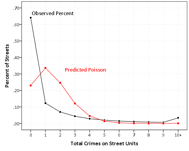
You then do this for not only the number of predicted zeroes, but the number for each regular integer value. That is you would do the same exercise for the number of 1's, the number of 2's, etc. Then you can make a graph of the observed number of whatever integer versus the predicted number. Here is an example graph with our original model using only the total number of alcohol outlets to predict the number of crimes on a street unit. You can see that the model under predicts the number of zeroes, and over predicts the number of higher integers. Here I just bin the integers that are 10 or more in the graph. In this chart the black line is the observed percentages in the data, and the red line is what our Poisson model predicts. You can see that the model predicts too few 0's and too many 1's, 2's and 3's. Also the number of 10+ appears to be too few.

To address this poor fit, the negative binomial model is the simplest extension of Poisson regression. It allows the variance to not be a function of the mean, but to vary with the mean. The most common form of negative binomial regression models set the mean to:

\[\mathbb{V}[Y_j] = \lambda_j \cdot (1 + \alpha \lambda_j)\]

Where \(\lambda_j\) is the predicted mean for the \(j\)th observation obtained from the usual Poisson regression equation, e.g. \(\lambda = \exp(\beta_0 + \beta_1X)\). For the negative binomial model the mean equation is exactly the same as Poisson regression (an exponential function of the inputs) but the variance is a function of both that mean plus a dispersion term, \(a\). Note that in the case that \(a = 0\), you get the usual relationship for the Poisson distribution that \(\mathbb{V}[Y_j] = \lambda_j\) - that is the variance equals the mean. So higher values of \(a\) mean the distribution is more overdispersed.

This is frequently referred to as the NB2 model, and is the default in most statistical software.² The mean equation is still the same in negative binomial models, so they tend to produce very similar coefficient estimates compared to Poisson (Berk and MacDonald 2008), but they will make the standard errors larger. I've only ever come across one example of crime data that was underdispersed. In that case negative binomial models are not applicable - they can only model overdispersion. See Sellers and Shmueli (2010) for an example of modeling underdispersed count data.

Now we need to do the same exercise with our overdispersed data as with our Poisson data. The formula for the PMF for the negative binomial distribution is much more complicated than that for the Poisson distribution. This formula is listed in Long (1997) and is below (here \(\hat{\lambda}\) is the predicted mean from your equation, and \(\hat{\alpha}\) is the overall dispersion term estimated for every observation):

\[\frac{ \Gamma(k + \hat{a}^{-1}) }{ k!\cdot \Gamma(\hat{a}^{-1}) } \left( \frac{\hat{a}^{-1}}{\hat{a}^{-1}+\hat{\lambda}}\right)^{\hat{a}^{-1}} \left( \frac{\hat{\lambda}}{\hat{a}^{-1}+\hat{\lambda}} \right)^k\]

Where \(\Gamma\) is the gamma function. Pretend we estimated a negative binomial regression model, and then had a dispersion estimate of 0.8, but the predicted means were exactly the same as the Poisson regression. Then for our first row, we would predict the probability mass for the number of zeroes as:

\[\frac{ \Gamma(0 + 0.8^{-1}) }{ 0!\cdot \Gamma(0.8^{-1}) } \left( \frac{0.8^{-1}}{0.8^{-1}+0.5}\right)^{0.8^{-1}} \left( \frac{0.5}{0.8^{-1}+0.5} \right)^0\]

Which in this case the first part with the Gamma functions and the last parentheses turn into one when examining k=0, so we are just left with the middle part (note that \(0.8^{-1}=1.25\) ), so we then have:

\[ \left ( \frac{1.25}{1.75} \right ) ^{1.25} \]

which equals about 0.66.

So going through the same motions for each row in our dataset,

C   l   P0   N0
0 0.5 0.61 0.66
0 1.0 0.37 0.48
2 3.0 0.05 0.22
3 2.0 0.14 0.30
5 4.0 0.02 0.17

Which adding up those five rows for N0 you then end up with 1.83, which divided by 5 equals 37%. So in this case having an overdispersion term of 0.8 gets us close to the same number of 0's in this very small example.

Extending this to our data, again with just using the number of alcohol licenses to predict the number of crimes on a street unit, we negative binomial regression we end up with the equation:

\[\log ( \mathbb{E}[\text{Crime}] )= 0.30 + 0.67\cdot(\text{Alcohol Lic.}) \]

And we have an estimate of the dispersion term as 4.5. Displaying our same chart of the observed proportion of integers versus that observed, we can see that the negative binomial model, with only one covariate in this case, fits the data near perfectly. The lines overlap so much I do not even know where to put my labels!

This is my experience - that the negative binomial tends to fit most crime count datasets quite well. Often people suggest to use zero-inflated (or other related models, like hurdle models) just because they see a high proportion of zeroes in the dataset. In this data even modeling burglaries on street units, which have nearly 90% zeroes, the negative binomial model fits quite well. Because of this I don't recommend zero-inflated models unless you have a strong theoretical reason - and I will go over some of those models in a later section.³

Using Offsets to Interpret Poisson Regression as Rates

When one is predicting crime counts, it is often the case that one wants to interpret the outcome in terms of rates per population, instead of just simply the counts. For instance, say one had counts of robberies at the city level, and one wanted to compare robbery rates per population between cities. This is easiest to accomplish in Poisson regression through an offset term (or sometimes in statistical software called an exposure term when dealing with Poisson data). An offset is just a term in a regression equation set to a specific value.

So starting with our original model, we will include a term that is the logarithm of the population. Imagine this as another coefficient, but its value is fixed to 1, instead of estimated via the data. So here is the regression predicting the expected number of crimes as an exponential function of some input variables, including the population of the area.

\[ \mathbb{E}[\text{Crime}] = \exp [ \beta_0 + \beta_1X + 1 \cdot \log ( \text{Population} ) ]\]

Note that you can rewrite the right hand side of this expression to be:

\[\exp [\beta_0 + \beta_1X] \cdot \exp [\log ( \text{Population} )]\]

And now divide each side of the equation by \(\exp [\log ( \text{Population} )]\) to then have:

\[ \frac{ \mathbb{E}[\text{Crime}] }{\exp [\log ( \text{Population} )]} = \exp [ \beta_0 + \beta_1X ]\]

Further note that \(\exp [\log ( \text{Population} )] = \text{Population}\), because the exponential and logarithmic functions are inverses of each other. So this means that by including an offset of the logged population, you can interpret the remaining coefficients as affecting crime rates per population.

\[ \frac{ \mathbb{E}[\text{Crime}] }{\text{Population}} = \exp [ \beta_0 + \beta_1X ]\]

Because the mean equations of Poisson and Negative Binomial models are the same, this interpretation holds for both.

So this shows why including an offset results in an interpretation in terms of rates, but then there are some practical questions that need to be addressed. One is that crime may not scale proportionally with the population size. It is often the case that rural areas have very low rates of violence compared to urban areas. This would suggest that the coefficient for the population should not be set to 1, but should be estimated via the data. Another is that the denominator for the rate can sometimes be arbitrary. For instance, if we are examining rapes should the denominator be the entire population - or should it be only the female population? For examples of non-traditional population denominators, you have cars for motor vehicle theft (Boggs 1965), the day-time population for cities (Stults and Hasbrouck 2015), or the number of potential pair-wise interactions for intra-racial violence (Hipp, Tita, and Boggess 2011). This choice is not trivial - choosing different denominators can impact the effect estimates for all of the other coefficients.

Often times there is no empirical way to say whether some denominator is more appropriate than others (Firebaugh and Gibbs 1985). Sometimes a more parsimonious model is to make all variables as rates per population, but you often cannot look at the numbers and say this model beats that model. It needs to be driven by how you theoretically expect the process to operate.

Additional notes are that you can incorporate multiple variables into one offset. Say you were examining the number of fights among different prison blocks, and you have measures of the number of inmates and the number of hours they served on a block. You would then use log(#inmates*hours on block) as the offset term. (Pretty much all rates have an implicit time component.)

Also it is the case that a linear transformation of the rates does not impact the coefficient estimates. So if you include log(Population) or log(Population/100,000) it does not make a difference for any covariates in the model besides the intercept term.

Comparing Error Distributions of Poisson, Negative Binomial, and Regression on Logged Outcomes

ToDo Wicklin blog post

Do I Need a Hurdle or Zero-Inflated Model?

ToDo - probably not

Further Notes on More Complicated Designs

There are several complications with extended Poisson regression to more interesting designs that take advantage of temporal or spatial aspects of the data. One is that endogenous lags are typically very bad for Poisson equations, and should be avoided. For a simple example, lets take the time series case and imagine a linear regression of the form:

Problems with Poisson Regression for Time Series Data

So start with a simple auto-regressive linear model:

\[Y_t = 0.5\cdot(Y_{t-1}) + \epsilon \]

So if you put a shock at time t=0 of 4, you will then have the subsequent predictions of:

\[ \begin{align*} Y_0 &= 4 \\ Y_1 &= 0.5\cdot 4 = 2 \\ Y_2 &= 0.5\cdot 2 = 1 \\ Y_3 &= 0.5 \cdot 1 = 0.5 \\ \end{align*} \]

Eventually that initial shock of 4 wears off. For linear equations, as long as the absolute value of the regression coefficient is less than 1, the shock will eventually die out, and hence the auto-regressive equation is not explosive.

This less than the absolute value of 1 rule does not work with Poisson regression though. Lets go through the same example, except with the exponential function for Poison regression:

\[Y_t = \exp( 0.5 \cdot (Y_{t-1}) + \epsilon )\]

We then have for our predictions by seeding the initial time period at 4:

\[ \begin{align*} Y_0 &= 4 \\ Y_1 &= \exp(0.5\cdot 4) \approx 7 \\ Y_2 &= \exp(0.5\cdot 7) \approx 40 \\ Y_3 &= \exp(0.5\cdot 40) \approx 485,165,195 \end{align*} \]

So you can see that a shock of 4 never wears off, and grows quite dramatically in only a few time periods. This is not a realistic time series model of how a Poisson process might go.

Unlike in linear regression, there is not a fixed coefficient at which a shock is not explosive. If you have \(a\) as the auto-regressive coefficient, then you basically need \(\exp(a\cdot y_{t-1}) < y_t\) for the endogenous lag to not be explosive. So this tends to need to be a really small auto-regressive effect. I give an example in Andrew P. Wheeler (2017), where I estimated an effect with this data of 0.08, and that was still explosive with this dataset. Because of this I suggest in that same article if you must, to include the logarithm of the endogenous crime counts. Which makes the equation much less likely to be explosive.

In the limit the shock will tend to never wear off (see here for an example). What this means is that auto-regressive Poisson processes are also non-stationary, even if they are not explosive.

Because of this you typically cannot estimate auto-regressive processes with Poisson data, either for univariate time series analysis or for panel data analysis. Although it is common in the field, it is almost always a mistake. See Brandt and Williams (2001) for applying time series models to Poisson regression equations. But some of those models are still not regularly implemented in statistical software. Also White, Porter, and Mazerolle (2013) have an example applying self-exciting point processes to terrorist data, which are Poisson models with a continuous auto-regressive parameter.

Poisson Regression With Spatial Data

ToDo spatial data (Bhati 2008; Lambert, Brown, and Florax 2010)

See this post for notes

See also self-exciting point-process models, e.g. Mohler et al. (2011) and Loeffler and Flaxman (2017). These are essentially auto-regressive Poisson processes (with AR in space and time). These are the models used in the PredPol predictive policing algorithm.

Poisson Regression With Panel Data

ToDo panel data - read Allison and Waterman (2002)

A Note on Differences in Differences with Poisson Regression

ToDo - see this blog post for now

Are Your Effects Really Exponential?

ToDo - See my dissertation for examples where effects are pretty linear. In particular Figure 15 (pg. 121), Fig. 16 (pg 122), and Figure 29 on pg 164.

Other Interesting Applications of the Poisson Distribution

• Capture/Recapture (Bouchard 2007; Rossmo and Routledge 1990), see also an attempt to measure the number of civilians killed by police using this method
• control charts with Poisson data (Andrew P Wheeler 2016)
• other operations research applications of Poisson data (Maltz 1996)

References