For a reminder, the readings for this week are:
In this weeks lecture notes we will be going over the journey to crime and practical applications of examining where specific offenders commit crime.
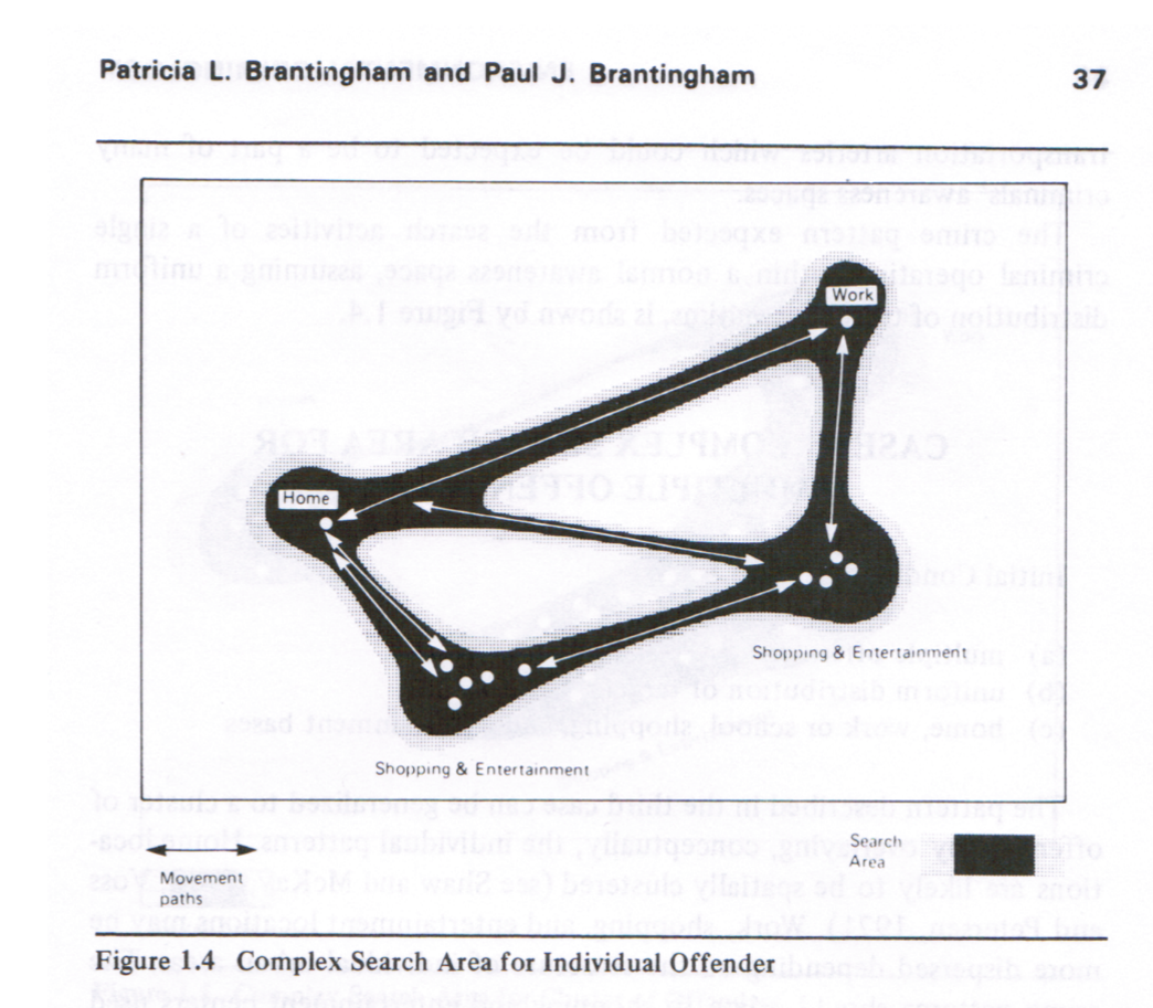
The journey to crime (JTC) is simply the distance between where an offender resides and the location they commit their crime. If you remember the idea of nodes and edges in crime pattern theory (P. L. Brantingham and Brantingham 1991), where an offender lives would be considered a node.
Places such as a favorite bar or where an offender works would be considered other nodes, and offenders become familiar with the places between those nodes from repeated traveling. An offender is more likely to commit crime at places they are familiar with for probably obvious reasons. In the case of expressive crimes (such as assault), this is due to simply their routine activities. Offenders probably do not go and look for a fight at special places beyond their normal hangouts. In the case of instrumental crimes (e.g. robbery, burglary), offenders are most likely to be familiar with potential targets in areas that they frequent. For example Rengert and Wasilchick (2000) interviewed burglars, and they said they would spot houses on the way to/from work that they would target.
Some have described the behavior of offenders as animals foraging (Johnson, Summers, and Pease 2009). For example, Jacobs (2010) described how chronic robbers have particular neighborhoods they are familiar with, but would cruise around in a vehicle looking for a particular mark to rob. So it was both partly planned, but subject to random opportunity factors as well. Comparing offender footprints (where offenders have committed crimes over time), tend to look quite similar to people who track animals, hence the relationship to ecology and foraging.
So there end up being two constraints in offender mobility – where actual opportunities to commit crime exist, and where offenders are familiar with. Even if an offender is familiar with a particular lake, there probably won’t be any opportunities to steal from individuals in the middle of it. It appears that most criminals subsequently use as little effort as possible to find victims, and this results in many short trips for the journey to crime. Here is an example from some of my work, (Wheeler 2012), for JTCs in Syracuse. The median crime trip from an offenders home location in this sample is 1.6 kilometers (this includes a sample of over 40,000 trips and all different crime types).
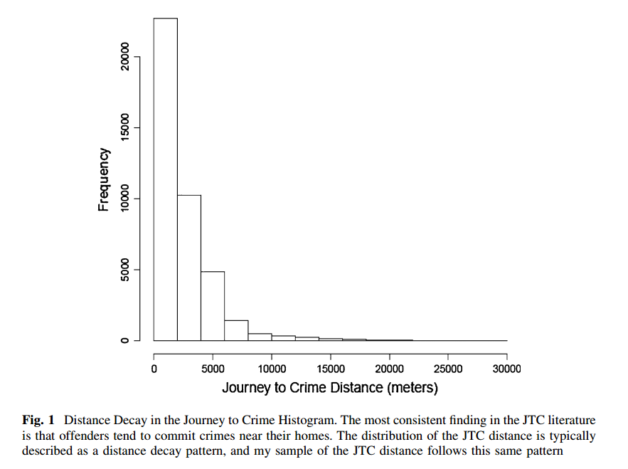
The pattern in this histogram, the heavy right skew, is described as distance decay – an offender is much more likely to commit crime closer to their home than farther away. This is one of the most consistent crime patterns in our field – this holds for pretty much every type of crime, every type of person, and in every city examined. Some crimes, people and places have longer or shorter trips on average, but this distance decay is still the predominate pattern.
Using the fact that the majority of journeys to crime tend to be short, Kim Rossmo came up with the idea of geographic offender profiling (GOP) (D. K. Rossmo 2000). The idea behind GOP is given a list of offenses you know are likely to be committed by the same offender (such as by a particular modus operandi), can you guess the most likely place for that offender to be living based on where those offenses took place? In practice this works very well for identifying some type of nodal point related to an offender. It may not be the actual home address (e.g. it may be a friends house or where they work), but there is quite a bit of confirmation that this technique works when we have data to verify in many situations. It surprisingly even works quite well with only a few offenses to work with, like around 5 linked offenses.
How this is useful is simply as a tool for detectives to limit the area where they might investigate possible suspects. Kim has a bit of a complicated formula to figure this out, and takes into account that offenders are likely to commit crime not too close to ones home. But in my opinion, simply just looking at the offense locations and picking the middle (Bennell et al. 2007) works almost as well (and is much less complicated). Hence why I had you read that Bennell paper. In practice as a crime analyst or detective you probably want to use all the data you have at your disposal. For example if you already have say a dozen suspects, you may want to prioritize those that live nearby the middle of all the crimes.
As an example of geographic profiling, Kim and company geoprofiled the location of Banksy graffiti locations in England (Hauge et al. 2016). For those not familiar, the artist is famous for graffiti paintings in public space that incorporate aspects of the built environment. Below is one example.
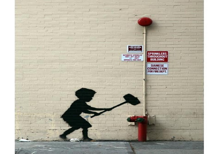
I grabbed some data of Banksy graffiti in New York City (via this Telegraph article for a place more familiar to folks in the class. While it is a bit lighter of a crime than most analysts are interested in, the logic works just the same. Kim subsequently gave his expert prediction using his GOP software.
First, here are the locations of those graffiti incidents in the city.
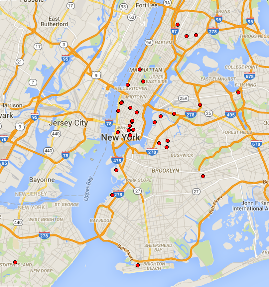
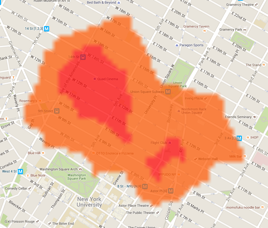
So we have a cluster in Manhattan, although there are some in each borough. This next image shows Kim’s prediction for the area that is 10% likely to contain the home address of the artist.

This is really too big to be useful, it includes pretty much all of lower Manhattan as well as a bit of Brooklyn, but you can basically see how the model is predicting based on essentially the middle of the incidents. The area in the center, the two darkest orange layers, are the places Kim labels as the top 0.1%. This ends up being pretty much on the border of Greenwich Village and the Chelsea neighborhood in lower Manhattan. While we do not know for sure the identity of the artist, this seems like a pretty reasonable guess. It is an area that has alot of artist type folks and college students with NYU, so there are quite a few apartments in the area.
So if you had no other information on who the offender was, that is the place you would begin your search.
While the journey to crime tends to be short, chronic offenders over time tend to display quite a bit of mobility. This may seem partly paradoxical, as the journey to crime is short. But what happens are some long journeys interspersed with short ones, as well as the fact that offenders move quite alot, results in chronic offender patterns encompassing large areas.
My favorite example of this is an offender who I will call Mr. Profilic, that came from my Syracuse project cited earlier. He was the offender that committed the most crime over the time period (he had 45 arrests over a 6 year period). Here are the locations of homes of the offender (in Blue diamonds) and offense locations (in red triangles).
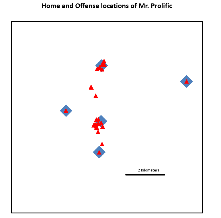
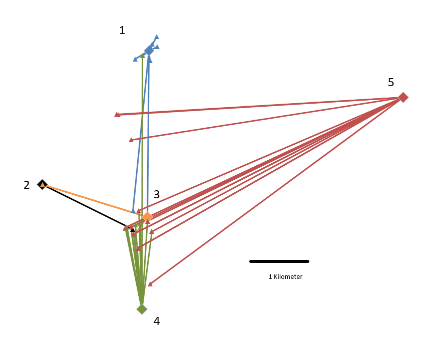
From this you would think that the journey to crime is quite short - but when I draw the actual trips another pattern occurs - the offender commits crimes by previous home addresses.

What happens over time is that the offender both commits crime at locations before he moves there, as well as re-visits old home locations. When he moves to the eastern part of the city, he ends up offending mostly back towards the central part of the city. The central part of the city is where most crime happens (not much happens in the eastern part, red below). So it is not clear for Mr. Prolific’s crime patterns if he is offending just where he hangs out (in bars in the central part of the city). Here the homes are labeled in their order, so you can see that he offenders nearby 3 when he lives at 1, and offenders nearby 2 when he lives at 3, etc.
As you can imagine with 45 arrests, they were not for very serious crimes. There are a few arrests for weapon possession and aggravated assault, but most are for nuisance crimes, like drunk in public or exposing himself to passersby. So many of the offense locations are more of the expressive variety.
Geographic offender profiling has the longest history/use in criminal justice, but there are several different types of predictions that crime analysts can use. These applications currently are not as simple as geographic offender profiling, but I think have good potential to expand going forward. Two of those applications are:
The Mike Porter paper I had you read was about predicting the location of the next criminal offense (Michael D. Porter and Reich 2012). While GOP tends to work well, this in practice tends to be much harder. Mike’s predictions ended up being on average 2 kilometers away from the previous offense. This matches up pretty well with my Syracuse sample - the inter-offense distance had a mean of nearly 2 kilometers (Wheeler 2012). Unlike how repeated offenses can give a clue as to the home offense, it does not appear that repeat offenses give new clues as to the next offense. I think this can be potentially improved though, using things like risk terrain modeling and/or discrete choice modeling (which we will read about next week).1
The second application is called crime linkage (Michael D Porter 2016). The idea behind this is that detectives have many unsolved crimes, each with a particular set of information. This information includes where and when the offense took place, as well as any peculiar modus operandi of the event (such as for a burglary the burglar entering the residence via pushing in a window AC unit). So the prior two applications (GOP and predicting the next crime), by necessity assume a series of crimes are linked to one another, crime linkage tries to identify those cases to begin with.
There can even be two distinct uses of crime linkage in crime analysis. One is that you have a known serial offender, and you attempt to identify whether cases of unknown origin are close to that specific offender. The other is more general, just in a batch of cases with unknown offender(s), can you identify any linked set of cases that are likely perpetrated by the same offender(s).
As an analyst, it is not easy to connect a serial offender, especially with fairly generic events for a large city. Even in a city like Troy, NY you will look at over a dozen burglaries per week. It is easy to miss small patterns that can potentially link those offenses together. Crime linkage is a way to identify cases likely to be linked - and being nearby in space and time is often one of the biggest factors in whether two crimes are related to the same offender.
For this weeks homework tutorial, you will be learning how to make multiple maps in ArcGIS, as well as a brief example of digitizing your own spatial data. The application will be mapping those same Banksy locations in NYC, as well as mapping a prolific offender and his journey to crime in Troy, NY.2
For next week we will be reading about two additional crime models: discrete choice models and geographically weighted regression. The readings for next week are:
Good luck on the homework!
Bennell, C, B Snook, PJ Taylor, and S Corey. 2007. “It’s No Riddle, Choose the Middle: The Effect of Number of Crimes and Topographical Detail on Police Officer Predictions of Serial Burglars’ Home Locations.” Criminal Justice and Behavior 34 (1): 119–32.
Brantingham, Patricia L., and Paul J. Brantingham. 1991. “Notes on the Geometry of Crime.” In Environmental Criminology, edited by Paul J. Brantingham and Patricia L. Brantingham, 27–54. Thousand Oaks, CA: Waveland Press.
Hauge, Michelle V., Mark D. Stevenson, D. Kim Rossmo, and Steven C. Le Comber. 2016. “Tagging Banksy: Using Geographic Profiling to Investigate a Modern Art Mystery.” Journal of Spatial Science 61 (6): 185–90.
Jacobs, Bruce A. 2010. “Serendipity in Robbery Target Selection.” The British Journal of Criminology 50 (3): 514–29.
Johnson, Shane D., Lucia Summers, and Ken Pease. 2009. “Offender as Forager: A Direct Test of the Boost Account of Victimization.” Journal of Quantitative Criminology 25 (2): 181–200.
Porter, Michael D. 2016. “A Statistical Approach to Crime Linkage.” The American Statistician 70 (2). Taylor & Francis: 152–65.
Porter, Michael D., and Brian J. Reich. 2012. “Evaluating Temporally Weighted Kernel Density Methods for Predicting the Next Event Location in a Series.” Annals of GIS 18 (3): 225–40.
Rengert, George F., and John Wasilchick. 2000. Suburban Buglary: A Tale of Two Suburbs. New York, NY: Charles C. Thomas.
Rossmo, D Kim. 2000. Geographic Profiling. Boca Raton, FL: CRC Press.
Wheeler, Andrew Palmer. 2012. “The Moving Home Effect: A Quasi Experiment Assessing Effect of Home Location on the Offence Location.” Journal of Quantitative Criminology 28 (4): 587–606.
———. 2015. “Visualization Techniques for Journey to Crime Flow Data.” Cartography and Geographic Information Science 42 (2): 149–61.
———. 2016. “Testing Serial Crime Events for Randomness in Day-of-Week Patterns with Small Samples.” Journal of Investigative Psychology and Offender Profiling, 13 (2): 148–65.
You might also ask when an offender will commit their next crime. I have not seen any work as to this question, but I do have a paper addressing whether repeated offenses are random with respect to the day of the week (Wheeler 2016). So this helps you decide if an offender is likely to commit their next crime on a Friday, or a Monday, or if there is no strong tendency to commit crime on any particular day of the week. This test I show in that article also only needs a few offenses, around 8 it is quite well powered.↩
I did not discuss cartographic aspects of displaying journey to crime data - but it is difficult. I do have an overview article discussing the challenges and presenting examples though in Wheeler (2015).↩