This tutorial goes over conducting spatial regressions in R. R is a statistical programming language. You can fit some of the same models in GeoDa I will show in this tutorial, but I typically fit such models in R. This tutorial is to get your feet wet with using R for conducting spatial data analysis, which has quite a bit more functionality for statistical analysis than any other mapping program. You can download the data used for this assignment from blackboard, or from dropbox via https://www.dropbox.com/s/nmle9smvs8k0xw1/8_SpatRegression.zip?dl=0.
The R program can be downloaded from https://www.r-project.org/. It should be also be installed on pretty much every machine in the SUNY Albany computer lab as well.
If you are interested in digging more into R, there are many different resources. For spatial data analysis there is a book I disseminated with your readings, Applied Spatial Data Analysis in R (Bivand, Pebesma, and Gómez-Rubio). They have a newer edition out, but it is a one stop shop for many of the types of spatial oriented regression models you can fit in R, along with notes on manipulating spatial objects.
Here I will first introduce how to install packages and interact with R. Then second I will show how to estimate a spatial lag regression model. In the extra notes at the end of the tutorial (which do not need to be done) I show how to read spatial data into R and estimate an alternative Poisson regression model that includes non-linear spatial terms. Also included in the data analysis are finished R scripts that show the same code. While you could simply copy and paste that, for learning it is better to recreate them on your own. They are there though to help troubleshoot if you have errors and cannot figure out what went wrong.
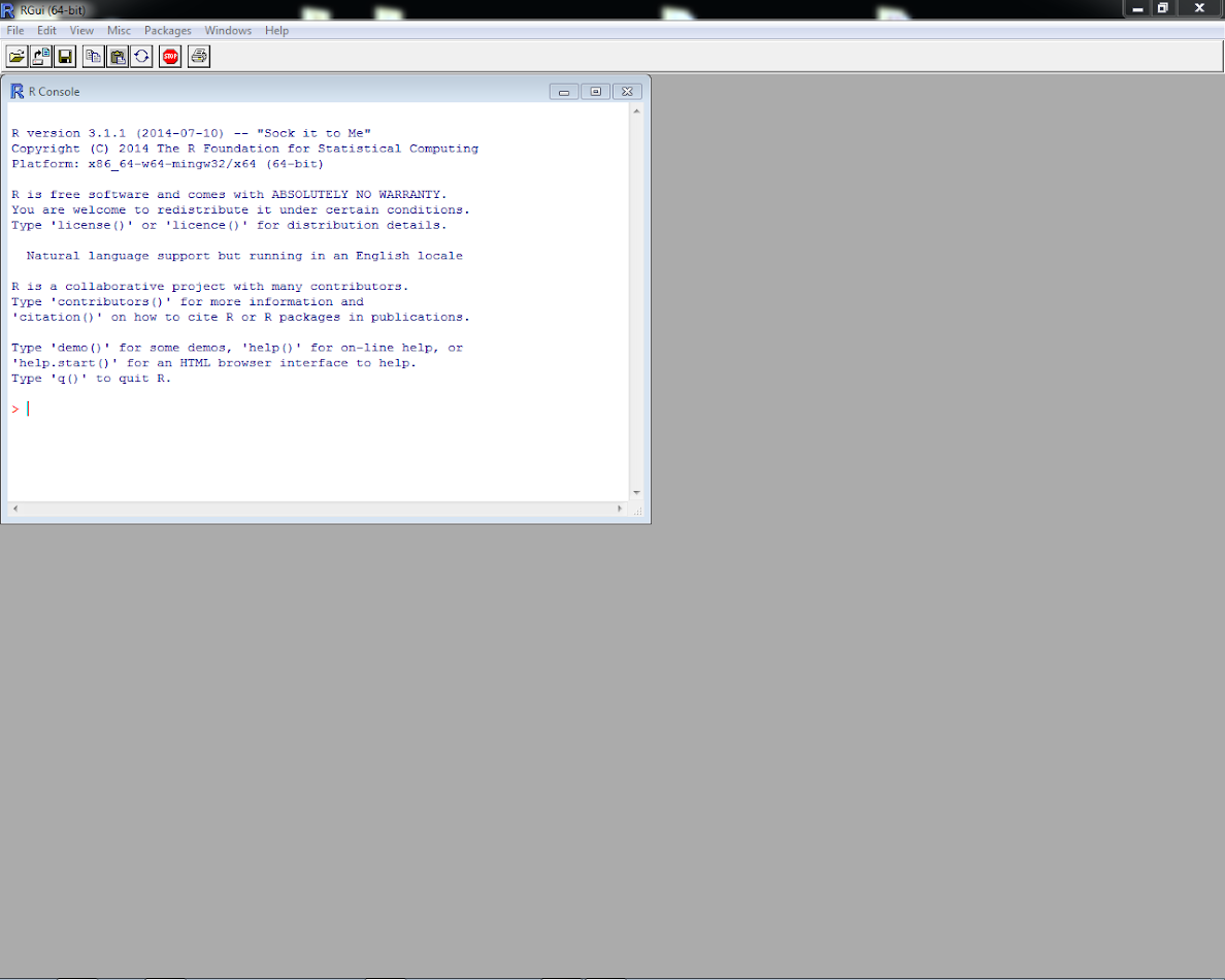
To open up R, navigate to the R folder (or program) in the program menu. If you have the option, feel free to select the Rx64 version. Once you open up R, your screen will look like below. (Note if you are using a personal machine you will have needed to install R.)
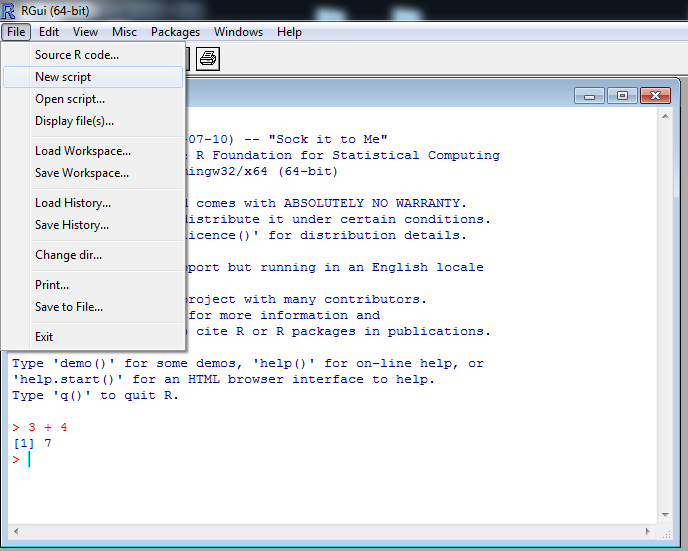
R has several windows. The one that is open is the console window. Go ahead and type 3 + 4 at the blinking cursor in the console window, then hit enter. R will then print back the answer.

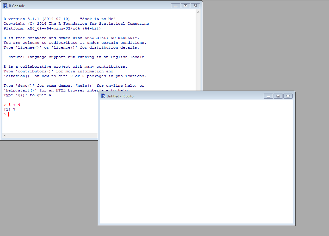
Now we are going to open up a new script window. Go to the File Menu and select New Script
You will then have a new blank script location. This is just a plain text editor, and can be moved around the space.
If you type in 2+3 in the script, highlight that line, and then hit enter it will populate the console with the command:
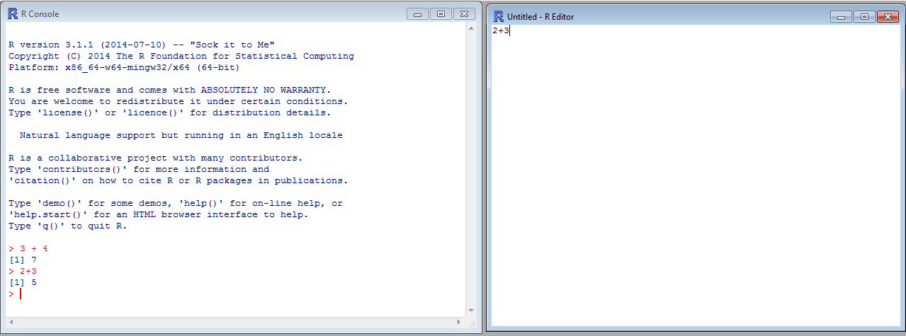
You can do commands either at the console or in the script. The script is better to save your results in the end to a file.
Now we are going to install some external libraries we will use in our subsequent analysis, specifically the spdep library. (It is supposed to be shorthand notation for spatial dependent variable.) Since R is free, many people contribute their own packages to extend the functionality of the software.
The typical code to install a particular package is install.packages("spdep"). But since you do not have write privileges on machines on campus, we are going to install the library to a location on your flash drive. So first create a variable that specifies the location that you have write privileges to - such as your flash drive.
MyDir <- "F:\\Spatial_Analysis_Course\\R_Lib"Note that I used double back slashes, this is because you need to escape the backslash - since it is a special character in some circumstances when R is deciding on how to interpret or print the string. R uses the <- symbol to mean assignment, whereas it uses = typically within function calls.
Now we are going to install the spdep library on our flash drive. With the command below:
install.packages("spdep",lib=MyDir)You will then get a prompt to select what mirror you want to download the package from. On Window’s machines I always have a hard time downloading things from the https servers, so I select a server in PA and then click ok.

R then proceeds to install the package and tells me everything is ok. Before exiting R, to search for the possible arguments to any function, you can simply type help(function) at the console, and it will bring up a help document file. So go ahead at type help(install.packages) at the console and see the example help page that is opened.
After you are done, go ahead and close R out. We will restart R and import these libraries in a new session.
Before we being estimating the spatial regression models, we will first load the spdep library that we just installed. Presuming you installed the libraries at a personal location, you can run syntax like below to load in the package. Note, you need to change the actual location of MyDir to wherever the library was installed on your computer or flash drive - e.g. it may be something like MyDir <- "E:\\GIS_in_CJ".
MyDir <- "C:\\Users\\andrew.wheeler\\Dropbox\\Classes\\SpatialAnalysis_Grad\\Lessons\\8_SpatRegression\\Lesson8_Data"
library(spdep,lib.loc=MyDir)
If you are on a personal machine that installed libraries to wherever the default location is, you can simply run library(spdep) and R automatically searches for the right location. Now we will set the working directory to the same location, MyDir, and then load in the RData file named “RurSpatData.RData”.
setwd(MyDir)
load("RurSpatData.RData")
ls()
The ls() command prints all of the objects currently available, which is now RurApp & QueenRur & MyDir. You made MyDir in this current section, but RurApp and QueenRur are new objects you loaded in. The first is a spatial data object of the counties, and the second is a spatial weights matrix made from a gal file from GeoDa. You can see the spatial object by using plot(RurApp), and see the variables available by using summary(RurApp).
Now we are going to check the amount of spatial autocorrelation in our outcome variables, LGVIOLRATE and LGPROPRATE. This data was taken from ICPSR study 3260, Spatial Analysis of Crime in Appalachia (1977-1996). What I did was take the average of the violent and property index crimes between 1988 through 1992 (5 years), and based on this average calculated the rate of crime per 1,000 individuals based on the 1990 census population. I then took the natural log of this variable, and this is what we will be predicting. So written out the dependent variable is:
\(\log(\frac{\text{Index Crime Counts}}{\text{Population}} \cdot 1000) = y\)
To check the spatial autocorrelation we will use the function moran.mc. But first we convert our neighbor file QueenRur into a format that many of the spdep functions need using the nb2listw function. (I also have commented out a way to make a contiguity matrix directly in R using the poly2nb function.)
#Many of the arguments require you to specify how the weights matrix is normalized
QueenList_RS <- nb2listw(QueenRur,style="W") #Type W is row standardized sums
#QueenList_RS <- nb2listw(poly2nb(RurApp),style="W") #To make contiguity neighbor directly in R
moran.mc(RurApp$LGVIOLRATE,QueenList_RS,nsim=999) #0.2316  - global Moran's I based on 999 permutations
moran.mc(RurApp$LGPROPRATE,QueenList_RS,nsim=999) #0.2837
Unlike say a simple t-test, the null distribution if the global Moran’s I coefficient is not easily determined. It is affected by both the nature of the spatial weights matrix and how the data is distributed. Because of these we use a permutation approach to artificially create the null distribution of the test statistic. We can see that for both property and violent crimes, there is quite a bit of spatial autocorrelation, much more than we would expect by chance.
It is possible we do not need to worry about spatial autocorrelation in the model if our explanatory variables are very good determinants of crime. Here we fit a simple linear regression model based on the variables:
BLACKPROP - the percentage of black residents in the countyEDULSHIGHP - the percentage of residents with less than a high school educationFAMPOVPROP - the percentage of families in povertyUEMPMALPRO - the percentage of males unemployedSo we can write out this linear regression model as:
\(\log(\frac{\text{Property Crime Counts}}{\text{Population}} \cdot 1000) = y\)
\(y = \beta_0 + \beta_1(\text{Black %}) + \beta_2(\text{Low Edu. %}) + \beta_3(\text{Pov. %}) + \beta_4(\text{Unemp. %}) + \epsilon\)
To estimate this model in R we can use the lm function, and the idiosyncratic way that you specify the regression formula in R is Y ~ X1 + X2 for the linear model \(Y = \beta_0 + \beta_1 X_1 + \beta_2 X_2 + \epsilon\).
#Simple linear model for property crime rate as a function of black % population, and % female headed households with children
Mod1 <- lm(LGPROPRATE ~ BLACKPROP + EDULSHIGHP + FAMPOVPROP + UEMPMALPRO, data=RurApp)
summary(Mod1)
You should then see in the output:
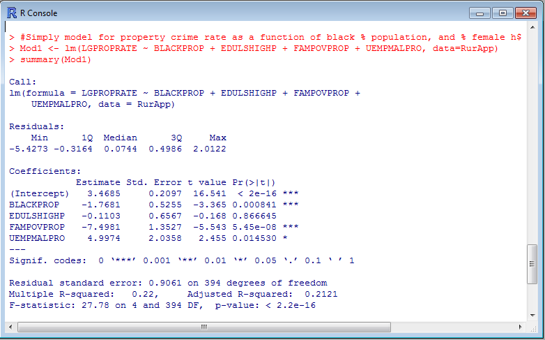
This gives you all of the usual stuff you want when interpreting a regression equation - both the coefficients and the model summary. Now we will check to see if the residuals still have any appreciable amount of spatial autocorrelation left in them using the same moran.mc function. To get the residuals of the model we can use residuals(Reg_Model_Object):
#can use residuals(Mod1) to grab them and check for spatial autocorrelation
moran.mc(residuals(Mod1),QueenList_RS,nsim=999)  #0.1567
We can see that while the amount of spatial autocorrelation has been reduced, initially from 0.28 to 0.16, this is still quite a bit. (Ignoring statistical significance, you probably want to aim for 0.05 or less.) Now we will fit a model with an endogenous spatial lag to attempt to account for this auto-correlation. Specifically the model can be written as:
\(y = \rho W y + \beta_0 + \beta_1(\text{Black %}) + \beta_2(\text{Low Edu. %}) + \beta_3(\text{Pov. %}) + \beta_4(\text{Unemp. %}) + \epsilon\)
So we include an endogenous spatial lag of the outcome variable y on the right hand side. This needs a special estimation procedure, so we cannot estimate this model using lm. The Land and Deane article was a critique of individuals who simply calculate Wy and include it on the right hand side. Note the two stage least squares procedure of Land and Deane is implemented in this same spdep package in the function stsls, but here we will use the maximum likelihood formula in the lagsarlm function.
Mod2 <- lagsarlm(LGPROPRATE ~ BLACKPROP + EDULSHIGHP + FAMPOVPROP + UEMPMALPRO, data=RurApp, listw=QueenList_RS)
summary(Mod2)
moran.mc(residuals(Mod2),QueenList_RS,nsim=999)
We can see in the regression summary output that the estimate of the spatial autocorrelation parameter is quite high, 0.32. Typically with positive spatial autocorrelation, inclusion of the endogenous spatial lag will result in coefficients closer to zero and larger standard errors, which is the same (with the exception of the education variable) here. The summary of the model gives a test for spatial autocorrelation in the residuals, but we also use here moran.mc again to give us the same conclusion. The spatial autocorrelation in the residuals is now 0.0147, which is within sampling error of randomness.
Now with a spatial lag model like this, the total impacts of any individual dependent variable are not simply encompassed by the regression coefficient. This is because if change one of the explanatory variables, you also change crime, which then diffuses to nearby areas. To estimate the total impact of a variable, the spdep library has a simple function called impacts.
impacts(Mod2,listw=QueenList_RS)Which subsequently gives us:

So interpreting the effects of the unemployment proportion, so holding all other variables constant, we subsequently have as the total effects of unemployment on property crimes.
\(\log(\frac{\text{Property Crime Counts}}{\text{Population}} \cdot 1000) = \text{fixed} + (6.17\cdot \text{Unemp %})\)
Let’s say we want to figure out a change in going from 15% poverty to 10% poverty in the crime rate, with setting the fixed value at 3 (\(\exp(3)\) ends up being very near the mean property crime rate in the sample, which is around 20 per 1,000 individuals). We would then have:
\(\log(\frac{\text{Property Crime Counts}}{\text{Population}} \cdot 1000) = 3 + 6.17 \cdot 0.15 = 3.9255\)
\(\log(\frac{\text{Property Crime Counts}}{\text{Population}} \cdot 1000) = 3 + 6.17 \cdot 0.10 = 3.617\)
These are in terms of log changes in property crime rates. To make these values easier to interpret, we need to exponentiate the resulting values, so we then have:
\(\exp(3.9255) = 50.68 = \frac{\text{Property Crime Counts}}{\text{Population}} \cdot 1000\)
\(\exp(3.617) = 37.23 = \frac{\text{Property Crime Counts}}{\text{Population}} \cdot 1000\)
So we have a total change of 50.68 - 37.23 = 13.45, a reduction of slightly over 13 part 1 property crimes per 1,000 population if we reduce the unemployment by 5%. You can do the same exercise decomposing these effects between local reductions in property crimes and reductions in property crimes for neighbors by substituting the direct and indirect effects into the equation instead of the total effects.
Estimate a spatial lag regression model for the outcome of logged violent crime rates using the same explanatory variables. In a word document, make a table that compares the regression coefficients and standard errors for the property crime model to the violent crime model. Use the moran.mc function to determine if the residual spatial autocorrelation has been reduced and whether it is still statistically significant in the model residuals. Write a paragraph describing the differences in inferences and estimates between the two models.
For 5 points extra credit, estimate the indirect spatial impacts of the explanatory variables and describe one variable in terms of the direct, indirect, and total number of crimes increased/reduced given a hypothetical set of inputs into the model. State these specifically in terms of changes in violent crime rate.
For the in-class tutorial I have you start with a spatial data and a weights matrix already imported into an R dataset. Also the models I have you fit in the R example can be easily fit in GeoDa (although the indirect impact estimates cannot be easily obtained). Here are two extra sets of notes for importing spatial data and fitting a Poisson spatial model if you want to know how to do that your your own work.
In R I use the rgdal library to read in spatial data, and the spdep library has a function to read spatial weights matrices from a gal file (a neighbor file we created with GeoDa last tutorial). So first we are going to load up the libraries rgdal and spdep.
library(rgdal)
library(spdep)
If you do not have rgdal installed, follow the same instructions at the beginning of the tutorial. If you are installing libraries on your flash drive, remember to specify lib.loc as well. Next we are going to set the working directory to where are spatial data files (shapefile and a gal file) are located.
MyDir <- "C:\\Users\\andrew.wheeler\\Dropbox\\Classes\\SpatialAnalysis_Grad\\Lessons\\8_SpatRegression\\Lesson8_Data"
setwd(MyDir)
Next we are going to read in our spatial data using the readOGR function. There are other packages to read spatial data, but rgdal is the most extensive and also imports the projection data.
#To read in shapefiles use "readORG"
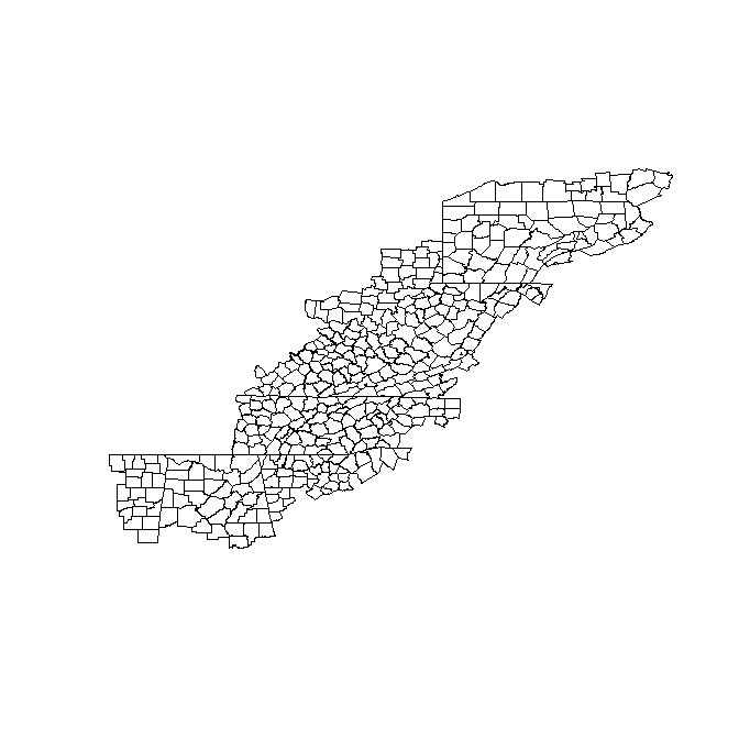
RurApp <- readOGR("RurApp.shp",layer="RurApp")
plot(RurApp) #Plot it to make sure it is okThe final line produces a simple map in R’s plotting window - this is a quick check to make sure everything is ok.
You can also see all of the variables importing by typing summary(RurApp) at the prompt. Next we will import the gal spatial weights file. To do this the spdep library has a function named read.gal.
#To read in the gal spatial weights matrix
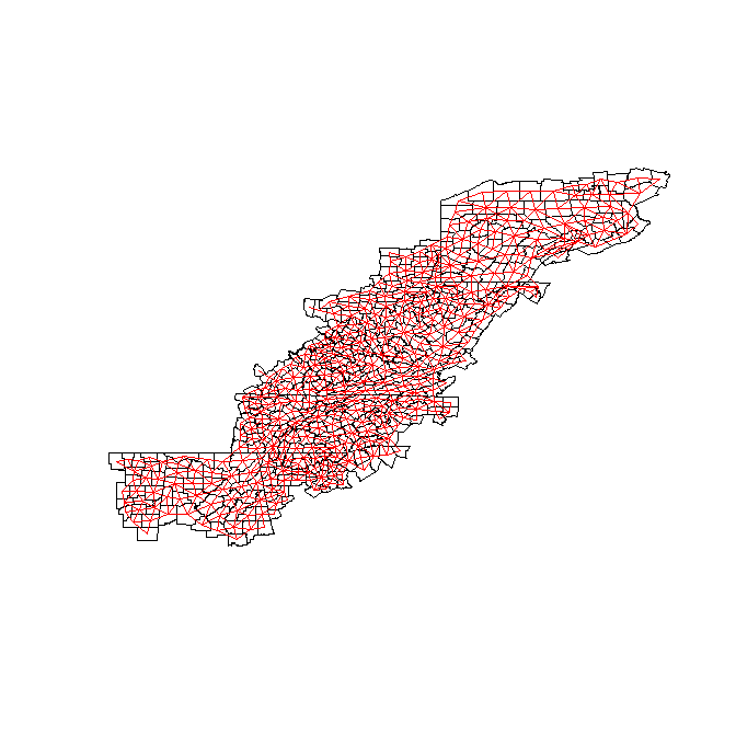
QueenRur <- read.gal(file="Queen1.gal",region.id=RurApp$FIPS_N)
summary(QueenRur)
plot(QueenRur,coordinates(RurApp),add=TRUE, points=FALSE, col='red')The line summary(QueenRur) prints out a brief description of the weights file, including the distribution of the number of neighbors. Similar to GeoDa, we can easily check to see that all units have at least one neighbor. R has default plot methods based on the object type, and here they have a nice connected plot made for the weights matrix. So we can see what neighbors are connected. The add=TRUE option specifies that it superimposes the plot over the prior outline map we made. Here is what that graph looks like now:
Finally we will save our file for future use.
save(RurApp,QueenRur,file="RurSpatData.RData")This saves it to the working directory.
For your tutorial I had you fit a linear regression model logged property crime rates. Often times, especially when predicting at micro places, linear regression is inappropriate because we have very many low counts. Here you will likely want a Poisson regression model, but you cannot fit an endogenous lag term in Poisson models easily.
An alternative then is to fit a Poisson model, but use non-linear terms based on the spatial coordinates. This is in effect very similar to a spatial error model. It also works quite easily for large datasets. Here we will use the mgcv R library to estimate the model, in particular it has a function called gam that estimates the smooth terms of the spatial locations automatically.
library(mgcv) #for fitting non-linear splines of coordinatesNow we will be working with the same RurApp data that we used in the homework. If you restarted your session, go ahead and redo the part where you change the working directory and load in the data. Then you can follow along below. First we will turn our data matrix from the RurApp object (a SpatialPolygonsDataFrame) into just a data frame with no associated spatial data.
RurApp_Data <- RurApp@data #Gets the data frame from the RurApp spatial data
xy <- coordinates(RurApp)  #gets the polygon centroids
RurApp_Data$X <- xy[,1]    #adds in the centroids into the RurApp_data
RurApp_Data$Y <- xy[,2]
RurApp_Data$Prop5 <- round(RurApp_Data$PIND_AV*5) #this is a fudge, since data won't exactly be integers
R with all its potential objects are incredibly complex. It just happens that SpatialObject@data is the right code to grab the data matrix from the original spatial data object. For most spatial data objects it is also the case that coordinates(SpatialObject) returns something - here for polygons it returns the midpoint (centroid) of each polygon. Then for our new object we created RurApp_Data we added two new columns, X and Y. Finally the data in our object is the average of property crime rates over 5 years most of the time, but some of the cases had missing data. Because of this I multiple by 5 and round the data to force it to be integers - what would happen with actually count data.
Next we will fit our Poisson model, including terms for the spatial locations.
PoisGamModel <- gam(formula=Prop5~ BLACKPROP + EDULSHIGHP + FAMPOVPROP + UEMPMALPRO + te(X,Y,k=5),
                    family=poisson,offset=log(TOTPOP90),data=RurApp_Data)  #fits tensor splines
Note you can wrap long commands on multiple lines in R. The formula is equivalent to lm(), except that we now have te(X,Y,k=5). This is a special term for gam, in which it fits the model based on tensor splines of the spatial locations with the interaction of 5 knots for each term - so 25 new terms that need to be estimated. You can estimate the tensor splines yourself and include them if you want, but gam has various nice functions to automate this for you.
We can subsequently see how much auto-correlation is in our residuals from this model now compared to our original data. Note the moran.mc function is from the spdep library, so that will need to be loaded.
moran.mc(RurApp_Data$Prop5,QueenList_RS,nsim=999) #Originally 0.0809
moran.mc(residuals(PoisGamModel),QueenList_RS,nsim=999) #reduced just a bit, to 0.0529
This dataset seems to be a very good example of using a spatial lag model, since the logged crime rates are close to normally distributed. My dissertation was a better example of using such smooth spatial terms though. So this is mainly for demonstration purposes (not that this is necessarily a better model given these circumstances).