For a reminder, the readings for this week are:
First, if you have not done so, take a few minutes to review the test from last week. The test is simple, but are core concepts you should be familiar with to be a competent crime mapper.
For this weeks lesson, we will discuss analyzing areal data, also sometimes called lattice data. This simply includes measures for spatial areas, such as census areas we have previously made for choropleth maps. These take a different set of procedures to analyze than do points patterns. For crime analysts, you may have aggregate statistics at police beats you want to analyze, or for researchers they often use census areas. People who conduct surveys sometimes can only survey individuals at the zip code level (through mailings). You can also analyze much smaller units, such as individual addresses, and much of my scholarly work splits the city up into streets and intersections.
Point pattern analysis (last lesson) is often just focused on analyzing one type of data, such as assaults or robberies. This weeks lesson will be focused on analyzing the correlations between different variables though.
My favorite example of explaining spatial effects is talking about bars and crime. Many people believe bars are more dangerous, and this is borne out in much research – bars tend to be places that have more crimes. You could get a sample of addresses in a city, and then look at the correlation of whether the address is a bar or not and the numbers of crimes committed there. You could fit a regression model, predicting the number of crimes at an address as a function of whether it is a bar, along with other factors such as the number of people who reside there, the age of the building, whether it is another type of commercial establishment, etc.
But the power in conducting spatial analysis is to examine the relationships between places. Places nearby one another interact with each other, and these spatial interactions and spill overs can help us better model whatever phenomenon that is under study. Continuing with the bars example, bars can both increase crime inside the bar, as well as increase crime around the bar outside. This can happen because people need to walk to and from the bar, and they are more exposed to some victimization (like robbery) outside of the bar.
So we may end up estimating an equation predicting the number of crimes on a street as something like:
\[\text{Crime on Street} = 2 \cdot (\text{Bars on Street}) \: + \: 1 \cdot (\text{Bars on Neighboring Streets})\]
So here we have if you live on Main St., if they add an additional bar to 1st St. it increases the total predicted number of crimes by 2 on 1st St. If they add a bar to 2nd St., it increases the total number of crimes on 1st St. by 1. This is a spatial spillover effect, and one of the fundamental reasons to be interested in spatial analysis.
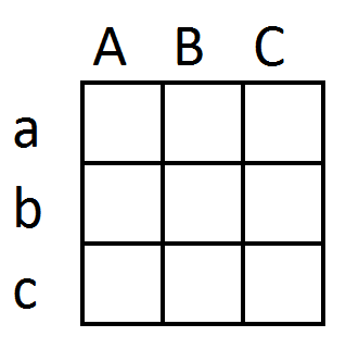
But how do we measure nearby in space? To do that, we need to define what exactly “neighboring” means in the above equation. When working with areal data there are a few different ways to define what neighbors are. The simplest and most often used is if two areas “touch”, they are neighbors. I will work through a simple example to illustrate. Pretend the simple grid below are the areas under study.
The individual units in this example can be defined by the row and column heading. So in a 3 by 3 grid we have 9 units of analysis.
Aa
Ab
Ac
Ba
Bb
Bc
Ca
Cb
Cc
So if we define neighbors to be touching only if they have a shared border, then Aa would have neighbors Ba and Ab.
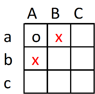
This is called Rook’s contiguity, for how a Rook moves on a chess board. There is another way to define touching though, including even if they only touch at a point. In this example that would make Bb also a neighbor of Aa, and that type of Contiguity is called Queen’s contiguity, for how a Queen moves on a chessboard.
There are additional ways to define neighbors beyond just simple contiguity. You may define neighbors based on a percentage of the total shared border, so two units that have a longer shared border (e.g. US and Mexico compared to Mexico and Guatemala). So although both are neighbors, in that example the US value would be weighted higher than the Guatemala value in calculations. You may define the closest 5 units to be neighbors, and that is called k-nearest neighbors (where you can fill in your own k). Another common way to define neighbors is via inverse distance weighting, where points nearer by one another have higher weights.
A fundamental aspect of estimating spatial relationships is calculating spatial lags. I will show this using our same small grid, but filling in these values.
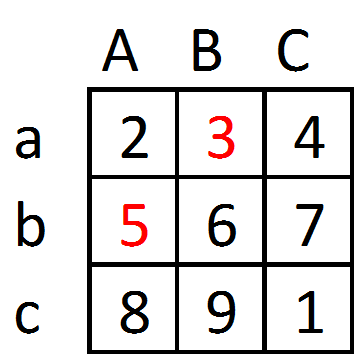
So in this example, the value at Aa is 2, and the neighboring values are 3 and 5 (using Rooks contiguity). We may be interested in the sum of the neighbors (8), or the average of the neighbors (4). But I am going to show a more general way to think about calculating spatial lags. So imagine that you have a spreadsheet, that in one column has the values, and in another column has a weight. Define the weight here to be equal to 1 when an observation neighbors Aa, and otherwise 0 (also we never define a unit to be a neighbor of itself). Then multiply the values times the weights, and sum that column. The sum of that column is simply the count of values in neighboring areas to Aa.
Unit Value Weight Value*Weight
Aa      2    0         0
Ab      5    1         5
Ac      8    0         0
Ba      3    1         3
Bb      6    0         0
Bc      9    0         0
Ca      4    0         0
Cb      7    0         0
Cc      1    0         0
------------------------
 Sum of Value*Weight = 8
You can refer to 8 as the spatial lag of Aa. Note that if you want the average of the neighbors, not the sum, you can simply change the weight. In that case, you want the weight to be 1/n, where n is the total number of neighbors. In this example, Aa only has two neighbors, so the weight would be 0.5, and the resulting sum would be 4.
Unit Value Weight Value*Weight
Aa      2    0         0
Ab      5    0.5       2.5
Ac      8    0         0
Ba      3    0.5       1.5
Bb      6    0         0
Bc      9    0         0
Ca      4    0         0
Cb      7    0         0
Cc      1    0         0
------------------------
 Sum of Value*Weight = 4
You can basically put any weights you want, so this should clear up how you can generalize to the differential weights example.
There is more general notation to calculate spatial lags for the entire sample than going through one individual set of neighbors at a time. And this is by referring to a spatial weights matrix. In our small grid example, we need a 9 by 9 matrix (because of the original 9 units), that encodes the spatial weights for all 9 units. Then each column and row defines the neighbor weights. Then you can calculate all of the spatial lags in one operation as:
\[ \begin{bmatrix} & Aa & Ab & Ac & Ba & Bb & Bc & Ca & Cb & Cc \\ Aa & 0 & 1 & 0 & 1 & 0 & 0 & 0 & 0 & 0 \\ Ab & 1 & 0 & 1 & 0 & 1 & 0 & 0 & 0 & 0 \\ Ac & 0 & 1 & 0 & 0 & 0 & 1 & 0 & 0 & 0 \\ Ba & 1 & 0 & 0 & 0 & 1 & 0 & 1 & 0 & 0 \\ Bb & 0 & 1 & 0 & 1 & 0 & 1 & 0 & 1 & 0 \\ Bc & 0 & 0 & 1 & 0 & 1 & 0 & 0 & 0 & 1 \\ Ca & 0 & 0 & 0 & 0 & 0 & 0 & 0 & 1 & 0 \\ Cb & 0 & 0 & 0 & 0 & 1 & 0 & 1 & 0 & 1 \\ Cc & 0 & 0 & 0 & 0 & 0 & 1 & 0 & 1 & 0 \end{bmatrix} \cdot \begin{bmatrix} V \\ 2 \\ 5 \\ 8 \\ 3 \\ 6 \\ 9 \\ 4 \\ 7 \\ 1 \\ \end{bmatrix} = \begin{bmatrix} V \text{ s. lag} \\ 8 \\ 16 \\ 14 \\ 12 \\ 24 \\ 15 \\ 10 \\ 11 \\ 16 \end{bmatrix} \]
In general, if we define our spatial weights matrix to be \(W\), and our set of values as a column vector \(x\), then post multiplying our spatial weights matrix by our column vector products a new vector of the spatial lags.
\[\text{Spatial Lag of} \: x = W\cdot x\]
This example the spatial weights matrix is a binary rooks contiguity matrix. So the spatial lags are the sums of neighboring values. Later on, I will refer to a row normalized spatial weights matrix. All this means is that the row sums are constrained to equal 1 in the spatial matrix. The effect this has is simple, it turns the spatial lag into an average of the neighboring values, instead of the sum.
While this example is based on areal units, you can generalize this to points in space that do not touch. One example project of mine recently was to examine surveys that were aggregated to the nearest intersection. So in that case I defined the spatial weights to be 1/(distance between intersections). This is called inverse distance weighting, and if you constrain the spatial weights matrix again so its rows sum to 1, the spatial lag then gives you the inverse distance weighted sum.
You can define the weights based on many different factors. When examining streets for example, I may define the weights be distance to get from one street to the next, as opposed to adjacency (Groff 2014). If you are examining nations, you may use some alternative to space value, such as the number of imports or the total immigration/emigration between two nations as the spatial weight. In practice, there often is not an empirical way to determine the best spatial weights matrix, so it needs to be defined based on how you think the units interact with one another. When examining spatial units though, fortunately many of these different ways to measure nearby in space often produce very similar estimates (Lesage and Pace 2010), so it is not too big a deal for conducting data analysis.
One of the most basic analyses you will often see is a calculation of Moran’s I. You can think of this as a measure of correlation, except it is a measure of the correlation between a variable and its spatial lag. This is basically used to see if a variable has any of those spatial effects or spatial spill-overs I was talking about previously. So if the bar spillover example is true, it would result in high crime areas being next to other high crime areas, and would result in spatial auto-correlation. There are other types of spatial effects that could result in spatial autocorrelation as well, such as if crime begets more crime. If the outcome is not spatially autocorrelated, we can then safely ignore any potential spatial effects and treat our data as if they are a sample of independent units.
To measure this spatial autocorrelation we most often use Moran’s I. The scary formula for Moran’s I is:
\[I = \frac{N}{\sum_i \sum_j w_{ij}} \cdot \frac{\sum_i \sum_j w_{ij}(X_i - \bar{X})(X_j - \bar{X})}{\sum_j (X_i - \bar{X})^2}\]
Where \(w_{ij}\) is the spatial weight between observations \(i\) and \(j\), \(N\) is the total number of observations, and \(X\) is the value we are estimating Moran’s I for. All the sums (the sigmas) just mean we are performing this operation over all pairwise observations, so we are comparing every unit to every other unit.
But the Anselin paper about local values lets us make it not so scary. First, if we z-score \(X\), this makes average of \(X\) (the \(\bar{X}\)) equal 0, so those terms drop out of the equation. Also this makes the variance of \(X\) equal to 1, which is the denominator in the second term in the equation.
The first term before the sum is the total number of observations divided by the sum of all the spatial weights. When we row-normalize a spatial weights matrix, the sum of the weights equals \(N\), so that term drops out of the equation entirely. So if we z-score \(X\) and row-normalize the spatial weights matrix, Moran’s I is then simply:
\[I = \sum_i \sum_j w_{ij}X_iX_j\]
Note for any one observation, \(i\), then the local Moran’s I value is:
\[I_i = \sum_j w_{ij}X_iX_j = X_i \cdot \sum_j w_{ij}X_j\]
Which the \(\sum_j w_{ij}X_j\) term is simply the spatial lag of \(X_i\). When you make the Moran’s I scatterplot, as illustrated in the different readings for this week, the X axis value is the Z score of the variable of interest, and the Y axis value is the average value of the neighboring z-scores for the variable of interest. These values are then used to make the High-High and Low-Low spatial clustering charts, and I have an example of that in your homework.
The sum of these local values are then the global Moran’s I. This is what is used to see if the data are spatially autocorrelated. Its expected value is \(-1/N\), so with a sample size of 50 observations, you would expect a Moran’s I value of \(-0.02\) if the data did not have any spatial patterning. The variance of this statistic is hard to construct in practice though, so we often do a permutation test to generate the distribution of the statistic under the null (as discussed in the Anselin Local I paper). The idea behind this is we take the observed data values and randomly assign them to spatial locations, then calculate Moran’s I. You do this randomization, say 99 times, and if the observed Moran’s I value is smaller or larger than any of the simulations, it is statistically significant with a p-value of < 0.01.
In my experience with crime as an outcome, the spatial autocorrelation is often positive, but not large. Typically between 0.20 and 0.05 for different models and different units. Some things though have much larger spatial effects, such as house prices (which can have autocorrelation values of 0.8 and larger).
For your tutorial and homework, I have you use a new software, GeoDa, to conduct some exploratory spatial data analysis. The dataset is from my dissertation, examining the correlates of crime at micro places in Washington, D.C. I have turned street midpoints and intersections into areas.
Groff, Elizabeth R. 2014. “Quantifying the Exposure of Street Segments to Drinking Places Nearby.” Journal of Quantitative Criminology 30 (3): 527–48.
Lesage, James, and R. Kelley Pace. 2010. “The Biggest Myth in Spatial Econometrics.” Available at Https://Papers.ssrn.com/Sol3/Papers.cfm?abstract_id=1725503.