Overview

This will be a walk through of using CrimeStat and ArcGIS to conduct point pattern analysis. I will show how to enter data into CrimeStat, how to identify repeat address locations, and how to create a kernel density surface. This will be illustrated using robberies from Troy in 2014. The data for use in this lecture can be downloaded from dropbox at https://www.dropbox.com/s/chtvx9br2u8peql/Lesson5_Tutorial.zip?dl=0 or via blackboard.

Importing data into CrimeStat

CrimeStat is a standalone tool, produced by Ned Levine and funded mainly through the National Institute of Justice. It is not like ArcGIS in that it cannot make maps itself, but it provides functionality to conduct various spatial analyses and create additional map files (which can subsequently be mapped in ArcGIS).

I have provided the CrimeStat.exe file in the spatial files for this tutorial (see the CrimeStatFiles folder). You can simply double click the CrimeStat.exe file to run the program. You do not need to install it. (For reference though, you can download the program and its documentation from http://www.nij.gov/topics/technology/maps/pages/crimestat.aspx.)

So double click the CrimeStat.exe file, and this is the screen when you first open the file.

Now click the Select Files button to import the X-Y crime data. You will then be brought up a file navigation dialogue.

Browse to the Rob14.dbf file in the spatial data file download for this week, and then hit open, which will insert the file into the dialogue.

Then hit OK, and your file will be inserted into CrimeStat.

And this is what the screen will look like now with the data.

Now we want to tell CrimeStat what fields correspond to the X-Y coordinates, and whether they are projected. So in the X and Y rows use the drop downs to select the appropriate fields in the DBF file, X_METERS and Y_METERS respectively. Then in the lower options select that the data is Projected and that the Data units are in Meters. You do not need to worry about the Time Unit.

In CrimeStat there are big tabs and little tabs. So far we were on the big tab Data Setup and the little tab Primary File. We are going to stay on the same big tab, but switch to the little tab Reference File.

Now what CrimeStat needs is to know the bounding box of the area you are interested in. You can input the lower left and upper right areas of Troy into the boxes. CrimeStat wants to create a regular grid of boxes, and the number of columns tells CrimeStat how big they will be. Fill in for Troy the numbers in the screen shot below. For the lower left 215000 429000 and for the upper right 219700 440250. In the number of columns option specify 94. This makes the grid cells approximately 50 square meters each. (Note you can hit Save and give this a name to use later if you close and reopen CrimeStat.)

Note figuring out the correct bounding box in CrimeStat is a common problem. To do this, you need to understand what projection your data are currently in, and the find out what the bounds of your data are. To do this in ArcMap, note you can hover over a point in the map view, and that coordinate is displayed int the lower right hand side of the map. You then need to make sure your points and your map are in the same projection, and then you can fill in the lower left and upper right coordinates you need to estimate the KDE in CrimeStat.

Now we are ready to generate the repeat address locations and kernel densities. First we will generate the repeat address locations. If you import the current DBF file of the original Robberies into ArcMap and plot them, they will have some points perfectly overlapping one another at repeat address locations (e.g. 102nd and 5th Ave is in there 2 times). What we can do in CrimeStat is create a file that specifies the spatial location and the number of times a robbery was committed at it.

Generating Repeat Locations

In CrimeStat navigate to the big tab Hot Spot Analysis, and the little tab ‘Hot Spot’ Analysis I. Toggle the Mode option on. Your screen should then look like below.

Now the Save result to… button should be ungreyed - meaning we can select it. Go ahead and push that button. This will bring up a dialog meant to save the resulting file. In the dropdown select DBF (it is the only option) and specify where you want to save the resulting DBF file. Here I name it “Rob_14_Mode”.

Then click ok, and back in the main CrimeStat window click the Compute button in the lower part of the window.

A dialog will come up saying if the procedure ran correctly and its results. It states that the robbery file has 110 incidents, and if you scroll down (scroll bar circled in red) you can see one location had 3 repeat robberies, and another 9 locations had 2 robberies.

Go ahead and close that dialog. You should then be back at the main CrimeStat window. Now we are going to map these repeat address robbery locations.

Mapping Repeat Locations

Open up a new ArcMap document, then add in the Troy outline. Style it so the fill is hollow, but the outline is a thick black line.

Now we are going to add in a basemap imagery from online sources. This is nice so we do not have to make our own styles for roadways and background imagery. We can just import it through online.

Go to File, then Add Data, then Basemap.

Select the Topographic map, and then click add. (Note if you want to print greyscale they have a few relevant options among these basemaps.)

Now your map should have a basemap that includes roads, rivers, and topographic features, as well as your Troy outline.

Next we are going to add in the DBF file of the repeat addresses we just created. Navigate to wherever you saved the file created by CrimeStat. Although I named the file “Rob_14_Mode” in CrimeStat, CrimeStat appended “Mode” to the beginning of the filename, and so it is named “ModeRob_14_Mode.dbf” in my screenshot.

Now right click on the table and select Display XY data…

ArcGIS is smart here and ends up filling in all of the fields we need by default. We typically need to specify the X and Y coordinates, and the projection the coordinates are in. But here they are all filled in for us, so we can go ahead and click OK.

Now are map will be filled in with the locations. Here we are going to use graduated symbols to show locations that have repeat addresses. Right click on the point layer that was just added (mine is named ModeRob_14_Mode Events), and go to properties. Navigate to the symbology tab (top), select Quantities in the left hand column, and then select Graduated Symbols, then in the Value field select FREQ. Each of these are circled in the screen shot below.

Instead of visualizing all of Troy, we are going to zoom into a smaller location using the magnifying glass with the + symbol. Now navigate to the layout view, and pick one of the clusters of robberies in the city. Here I pick the area North of Hoosick St and going into Lansingburgh (which starts at 101st St.). I also placed several guides into the map, I want to leave extra room for my legend and title outside of the map plot area. Here is what my map looks like after these steps.

The robberies are somewhat small and don’t stand out much. So I am going to go back to the symbol properties. Select the symbol size to be from 10 to 32 (outlined in blue) and then edit the properties for all symbols (same as the outlines for the polygons last week - where to click is outlined in blue) so all of the points are bright red. Now here is what my map looks like.

Now we are now going to add in a legend with multiple items. In the file menu go to Insert, then select Legend. In the legend wizard Troy’s outline along with the Point pattern layer will be selected. Hit Preview, and you will see a legend added into the map.

Don’t worry about going through the rest of the wizard, and go ahead and click Finish. Now drag the legend outside the map area so it is easier to visualize it.

Now double click on the legend. This brings up a dialog that we can edit parts of the legend. First in the General tab make sure the Title part is detoggled so there is no default “Legend” title.

Now navigate to the Items tab in the Legend Properties dialog. Make sure the robbery point pattern is selected, and then click the Style… button at the bottom of the window.

This allows us to choose different sets of information that is displayed and how it is displayed in the legend. Select the Option that is in the second column three rows down.

Click OK, and you will be back to the Legend Properties box. Next, select the TroyOutline layer, and in the Item Columns area toggle the option “Place item(s) in a new column”. Hit the Apply button and you can see how the legend changes.

Now edit the text in the table of contents so the named map layers are nicer. Also add in the additional map necessities, such as a scale bar, north arrow, and title for the map. Also add in your name, and make sure to save your map periodically. Here is what my final map exported to a PNG file looks like.

Generating and Mapping Kernel Densities

Go back to crimestat, now we will be estimating a smooth kernel density estimate of the point pattern. Before moving on make sure to un-toggle the Mode option. (If you don’t do this, when you hit Compute again - for any procedure - it will recalculate the Mode file.)

Now navigate to the big tab Spatial Modeling I, and the little tab Interpolation I.

Click the Single Kernel density estimate button, and then the dropdowns below will turn on so you can manipulate them.

Now these options change how the kernel density is calculated. To explain what a kernel density is - imagine that each crime point is a ball of playdough. In a normal map, you cannot see when the balls are repeatedly stacked directly on top of one another with your birds eye view.

So what the kernel density estimate (KDE) does is smooths those little balls into mounds. Then we do this for every crime, and what we then show in the map is the thickness of all those overlapping mounds of playdough. Places that have many crimes nearby one another will have many mounds of playdough overlapping, and so will have thicker, e.g. more dense, and will be shown as darker colors typically in KDE maps.

The options below specify how exactly the little mounds of playdough are smoothed out, and then how the thickness of the playdough is measured.

As a brief ado about them:

• Method of interpolation: In my playdough analogy, this dictates the shape of the mound. E.g. it can be like a triangle, or like a flat disc (uniform). Normal, quartic, and exponential all look like smooth hills, but each has different slopes for how steep the hill is. This choice matters very little compared to the bandwidth – I typically just stick with the default Normal, although any except uniform would typically result in the same general patterns.
• Choice of Bandwidth: In the playdough analogy, this corresponds to how far to smooth the ball out. The default is an adaptive bandwidth, which means you find the distance to the N nearest neighbors, and spread the mound out over that radius. I pretty much always change this to a fixed radius, typically around 300 to 500 meters. The smaller the bandwidth, the more hilly the map will be, as the mounds will not overlap except when they occur at the exact same location. If the bandwidth is too large, it will smooth the map into one giant hot spot.
• Area units: Points per: This only matters if you specific Relative Densities in the next option. I typically do not use relative densities - so this does not matter. This specifies how to measure the thickness of the playdough. Basically you will export a thickness measure to every grid cell over the city. You can imagine as a ratio of thickness/area. It is hard to compare maps that have grid cells of different areas, so to make it easier to interpret, sometimes people normalize the estimates to be per some standard area, like a square kilometer. So if the thickness ends up being 2 crimes, and your grid cells are 50 square meters, the measure would be 2/(50*50). To normalize this to a square kilometer, you would multiple by 1000*1000, which ends up being 800 crimes. This is useful if you plan to compare to other peoples kernel density estimates, say a KDE in Albany, as it does not matter what the end size of the grid cells are. If you want to compare to other KDE’s with different grid cell sizes it is much harder to use absolute densities or percentages.
• Output units: There are three options, absolute, relative and probabilities. For absolute the grid cells all add up the total number of crimes in the sample. For probabilities, the grid cells all add up to 1. For relative, it is the absolute densities divided by the area and multiplied by a constant as mentioned above to make them comparable. I typically use Probabilities, as it makes different samples using the same grid comparable. All three options will produce the same shape of the KDE, it is just what the units mean exactly.

To continue on, fill in the options like I have below. It would be reasonable to use Absolute densities here, comparing robberies directly between the two years (there are 110 in the 2014 sample and 142 in the 2015 sample). But if you are say comparing robberies to burglaries probabilities would likely make more sense.

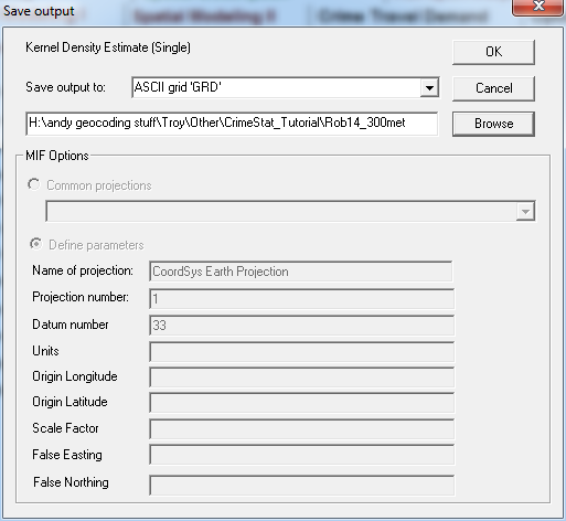
Now click on the Save Results To button to specify where we are going to save the kernel density estimate. Here I choose the ASCII grid format, and name the file Rob14_300met, so later I know it is the year 2014 and the 300 meter bandwidth version.

Then click OK, and you will be back at the prior screen. Now click the Compute button and a summary computation screen will pop up. If you scroll down and see that numbers are populated in the probabilities part you know it worked out. If these are all zeroes something somewhere messed up. My two most common errors are not specifying the background grid properly, or having problems exporting the data correctly.

Now we can import the grid into ArcMap and visualize it. Before doing that though, close out the computation summary window and go back to CrimeStat. Then click off the Single button. The reason for this is if you go and do some other computations in CrimeStat, if you don’t unclick that button it will redo the same procedure, and will overwrite the same file.

Now we can open ArcMap and make a nice map of the kernel density. You add the KDE to ArcGIS the same you do any layer, click the + button and import the grd file we just made (you will get a warning about the projection - ignore it and click ok). Then zoom back out so you can see the entire city of Troy, and toggle off the Robbery point pattern. Here is what my default looks like. ¹

The default map looks ugly, so we will work on making it look nicer. Right click on the layer in the table of contents, and then click properties. Go to the Symbology tab, and then click Classified. In ArcGIS V10 this causes an error.

Before we move on, we need to calculate statistics for the raster dataset. (Older versions it did this step for you automatically, it may do this automatically for you in the current V10.4.) In the toolbar click the Red Toolbox icon (highlighted) and this opens up a large set of commands in what is called ArcToolbox. Navigate to Data Management -> Raster -> Raster Properties, and then double click on Calculate Statistics.

In the dialog that pops up, populate the Input Raster Dataset field with the raster grid we are working with, and then press OK. (No other options are needed.) It will take a few seconds to compute. ²

Close out the ArcToolbox window, and then you can go back to the properties for the kernel density estimate to change the colors. Now in the Layer properties, select 4 classes, and in the Color Ramp dropdown select the second option (light to dark purple).

Now we are going to format the labels as percentages that sum to 100%. Click the table header for Format labels, and then in the dialog that pops up, select Percentage and then the option The number represents a fraction.... Then click the Numeric Options dialog.

Select the number of decimal places to be 3, and then click ok. Same as choropleth maps, where to make the breaks and how to do the colors is arbitrary. My guiding principal is I don’t want the whole map to be a hot spot - I want to focus on the very worst locations. Here I change the breaks to be nice guidelines as 0.01%, 0.02% etc. (shown last week in the classify dialog), and for the lowest color swath change it to be no color. After hitting apply here is what my breaks and map look like.

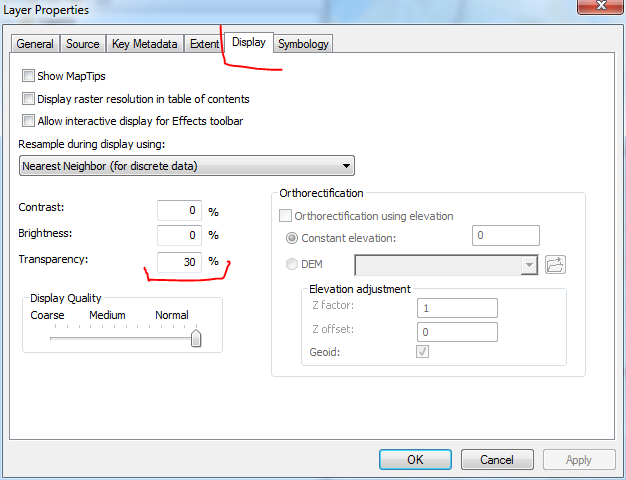
For the last part, we are going to make the KDE semi-transparent, so we can see the layers underneath it. Go to the display tab, and in the transparency box input 30.

Now you have your kernel density estimate and we can move onto making a nice map. In the layout view, add a scale. Also add a footnote describing how the KDE has calculated, which should include the bandwidth, kernel used, and the size of the raster cells. (When using relative densities the size of the grid cell does not matter, but when using absolute and percentages it does, so that is essential information in this example.) Finally add a legend that includes the kernel density estimate and the Troy outline. Place the Troy outline in a second column.

After those steps, your map should look sometime like this:

Next I want you to add a border to the outside of the legend. Double click on the legend area, and this brings up the Legend Properties box, and then select the Frame tab. In the dropdown for the border select the 1.5 width. The Legend Properties Screen should look like below.

Hit the apply button, and then look at the legend. You should notice a problem with the legend border – it overlaps the Troy outline, and butts up against the kernel density estimate swaths as well.

To fix this, go back to the Legend Properties screen. Below the border, set the Gap for X and Y to be 8, then hit apply. You can see now that the border has been expanded so it is not overlapping several of the parts of the map.

Probably the item students get the most points taken off for graded maps during the course are not editing the legend properly. Take care when doing this, as it makes your map look much more professional.

STAC Hotspots in CrimeStat

What follows is a tutorial on how to create arbitrary hot spot areas using one tool in CrimeStat, STAC. STAC stands for spatial and temporal analysis of crime - although this is a bit misleading, as it does not take time into account. The STAC procedure is what is called a spatial scan statistic (there is another popular called SatScan, I provide some notes on that at the end of next weeks tutorial). There are other clustering tools (I discussed k-means and hierarchical clustering in the lecture notes), but in my experience STAC provides the most reasonable output. It also has a simulation procedure to determine whether the hot spots would not be simply found by chance, which the other procedures do not.

First I am going to show you how to figure out the necessary bounding box though you need to use CrimeStat. Second I will show you how to calculate hot spot polygons in CrimeStat.

Figuring out the bounding box for CrimeStat

In the tutorial on point pattern analysis I showed you how to calculate a kernel density map using CrimeStat. To do this, you needed to import the bounding box you wanted CrimeStat to calculate the data for though – how do you figure that out for yourself?

Start a new mxd document, then import the polygon that is the outline for Philadephia, City_Limits_Proj.shp. My screen shot does not show my mouse, but the coordinates listed in the lower right corner of the map correspond to where the mouse is currently hovered over the map (those particular coordinates are somewhere within Philadelphia).

It is simple to figure out the bounding box then - just hover your mouse over the lower left point you want the resulting study area to cover and record that number, then hover your mouse over the top right coordinate you want to cover. This gives me something like [817,000 62,000] for the lower left, and [839,000 93,000] for the upper right. Here you do not need to do this, but I will show you quickly how to change these coordinates to the ones you need in CrimeStat (say if they currently display decimal degrees, and you need the projected meters). So in the Table of Contents right click on the top most Layers icon, then select properties.

Go to the general tab, and in the units section select the projected coordinates you want, here we just want to keep it at meters.

Note if your map is currently not projected it may not let you choose any reference system besides decimal degrees. See the tutorial on Map Aesthetics on how to change the overall projection the entire map is in.

Pro-tip: Another way to figure out the appropriate bounding box is to select a polygon that covers you area - here the outline of Philadelphia, and then right click and go to properties and then go to the source tab. It gives the bounding box of the coordinates on this tab - which you can my chosen coordinates by hand are just slightly rounded up or down from those coordinates.

Estimating STAC hot spots

So now that we have our bounding box coordinates, we can use CrimeStat. Go ahead and open up CrimeStat, and then import the dbf file from the “PhilShootings_LatLon” shapefile. Select the XMeters and YMeters for the X and Y fields respectively, and set the data units to meters. This should be on the big tab Data Setup and little table Primary File. (I will show in the tutorial next week how to create such fields on your own, e.g. if you download data and it only has lat-lon, but you want the projected meters for analysis.)

Now select the little tab Reference File (still on the big tab Data Setup). Input the lower left and upper right coordinates we just talked about. Here I also make the cell space (the size of the grid cells for kernel densities) equal to 100. Which if we were making a KDE it would make the resulting grid cell sizes 100 by 100 meters. We won’t end up using this information now though. Go ahead and save that specification as “Philly_Meter” for later use.

Now go to the big tab “Hot Spot Analysis”, and select the little tab “‘Hot Spot’ Analysis II”. (Please don’t perpetuate the scare quotes around hot spots – it is fine to just type hot spots or hotspots or whatever - we all know what you are talking about!) First click on the STAC option, then change the Output unit to Meters, and then click on the STAC Parameters button.

When doing these parameters for hot spots they are ultimately arbitrary - whether for STAC or whatever clustering routine you are using. So you may need to experiment with reasonable parameters. Here I set the search radius to 1,000 meters, set the minimum number of points to return a cluster to 30, set the simulation runs to 99, the scan type to triangle, and the boundary from the reference file. So here are what my final settings look like:

Once that is done click OK. Now we are back at the Hot Spot II little tab and the Hot Spot Analysis big tab. Now select the button Save convex hull to….. You will then get an output that should look similar to when you created your KDE. I’m going to save this as a shapefile with an informative name, “Tr_30_1000m”, so I can remember the parameters I used.

Once that is filled in, hit ok, and then hit compute. The screen will flash the simulations by a mile a minute, and then you will be done. You can scroll down the results to see that the procedure found 10 clusters, with one cluster having over 200 shootings in it. When conducting simulations, the simulated datasets did not return any clusters. (There is a stochastic element to this, your simulation may find clusters, mine did on earlier runs.) To interpret these basically if the simulations of random data do find clusters, you should be wary of using them in subsequent analysis. It reports the cluster sizes by the number of points, which in some of my runs do exceed 30 points. So I only want to focus on clusters that have clearly more than 30 points in my analysis.)

Now you can quit CrimeStat and head back to ArcMap. Import the shapefile of the hot spots you just made. The map should then look like below.

You can open up the attribute table and see how many points are in each cluster. For this example the clusters have nice shapes, so if you used ellipses instead of convex hulls they map might look a big nicer (but I think the convex hulls are more true to the data and better representations).

Before we are done though I have one more task though!

Assigning a Projection to the output from CrimeStat

In this example our STAC hot spots lined right up on our map. Sometimes this does not happen though output from CrimeStat. This is because output from CrimeStat lacks projection information - so if the map was in a different projection, when you open it up the polygons or kernel density or whatever may not line up with the other background information. To fix this, in the main file menu, select Windows and then select Search. (Note, if you ever lose your Table of Contents, you would select Table of Contents in this dropdown to get it back.)

This opens up a Search tab on the right hand side of your map. Search “project”, and then select the Define Projection (Data Management) little hammer, that is the tool we want in the end.

In the Define Projection window that popped up, select the STAC hot spot layer, and then we need to define the Coordinate System by clicking the button circled in red below.

This tab should now look familiar. Here we are using the same coordinate system as defined by the “City_Limits_Proj” shapefile. So click on the little globe with the graticule, and then click Import.

Navigate to the “City_Limits_Proj” shapefile and select that. Once you hit add, that projection, NAD_1983_StatePlane_Pennsylvania_South_FIPS_3702 should be there in the Favorites folder. (I have a bunch of additional projections in my screenshot that may not be in yours in however.)

Once that is selected hit ok, and you should now see that coordinate system populated in the Define Projection window.

Go ahead and hit OK. You won’t notice any physical change on your map, but if you go to the folder where you saved the STAC hotspot shapefile, you will now see that there is a “CSTTr_30_1000m.prj” file that was not there before. That defines the projection.

So if you are using CrimeStat and your data is not lining up - define the projection!

Pro-Tip: When displaying these arbitrary polygons, I often find it easier to make them as hollow fills, and then just a thicker black or red outline. That way you can see what is underneath, but they still pop out more.

Homework

Generate two out of the three types of hot spots I showed in the tutorial for the 2015 Troy robbery data: a repeat address map, a kernel density, or a STAC hot spot polygon. If doing a kernel density map, choose the bandwidth so it is only 150 meters, and select absolute densities. (Note you cannot then interpret them on a percentage scale, so do not make the legend to show percentages.) Make a map of the entire city, and replace the topographic basemap with the light grey base map. Edit your name into the map, along with all the other map essentials (title, legend, etc.), export it to a PDF file and turn it in.