
Here I am going to show an introduction to pivot tables in Excel. This is a reduced set of data of crimes in selected TAAG areas in Dallas in 2017. (TAAG stands for Target Area Action Grid, and they are meant as a sort of identified hot spot of crime by the DPD.)
If you took my Communities & Crime class it should look familiar – it is the data I gave you for your presentations. There I gave you the final Excel spreadsheet with all the nice graphs already. Here I am going to show you how to make it yourself.
You can download the original CSV data to follow along from ELearning, or from this link.
First, you should have downloaded a CSV file (linked above). It is named Lab02_TAAG_Areas.csv. (CSV stands for comma separated values, it is a plain text file format.) On my computer if I just double-click the file, it will open up in Excel. If this does not work, use right click and open in Excel.
Here is what the file looks like when I open it.
Select the cell A1, and then in the top toolbar navigate to the Insert tab. Then select the Table button.

You should get alittle pop-up window that automatically figures out where your data is in the sheet. Make sure the option My table has headers is checked, and then click OK.

You will see your table now is nicely formatted using zebra-stripes, and has little triangle icons at the top of each row. Select the ICON for UCROffense (column I). Then click off the Select All option, and then click on the Animal Bit option.

Once done, you will see that the sheet now only has the rows selected that have the crime type listed as an ANIMAL BITE.

Now go back and make sure all of the UCR categories are selected.

And the sheet should now be back to how it was to begin with. Then select the IncidentAddress header (column E). This time select the option to sort the rows, A to Z. (Also note you could use a simple search tool to look for a particular address.)

Via sorting and filtering, it is an easy way to conduct some simple data mining type analysis. Here we can see that 100 CRESCENT CT is a repeat crime address with a few assaults plus other junk. A quick google search shows it is a mixed office/food location.

The above approach is great when looking at individual incidents, but if you want to answer a question like “how many assaults occurred in January” or “what is the most common crime type in the Jefferson corridor area”. To do that, we are going to create what is called a Pivot Table. It allows us to make aggregations of multiple incidents, and estimate different quantities.
In the top tool bar, select the Insert button, and then click the PivotTable option.

You get a nice little pop up, and it should default to selecting the Table you already created. You can just keep all of the defaults, and select to put the Pivot Table in a new worksheet.

Once you hit OK, it should look something like this in the worksheet:

Next, in the right hand section, drag the field UCROffense down to the rows area on the right hand side.

Next, drag the UCROffense field again into the Values box in the lower left. This by default will give you the total Counts of UCR offenses in the Pivot table.

You can do other data summaries besides counts, like if you had a dataset of thefts, and you had a field of the estimated value of items stolen. In that case you could do a summary statistic like the average (mean) of those values. I use pivot tables mostly for counts though.
Next, drag the Day1oftheWeek field into the Columns area. You will then see the counts are further broken down by each day of the week.
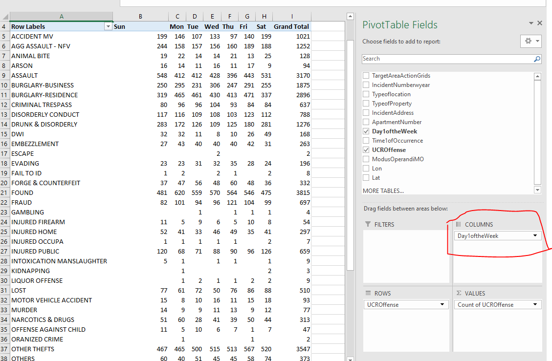
For the last part, drag down the TargetAreaActionGrids field into the Filters area. Then above the table you will see an extra row with the same type of dropdown as the table with the original incidents.

Select that dropdown, and then click the Coit Churchill+ option.

You can see now that the total numbers are much lower. They now only include those cases that occur within that particular area.
We can create graphs with the Pivot Table data the same as we did in the first week. But, with the pivot table we can do what are called slicers in the chart. Basically how we can filter the pivot table data, we can have that same behavior tied to a chart. Clear out the variables in the Pivot Table (just drag the variables outside of the window they are in, or select the field and click the Remove Field option). Then redo the pivot table so it is TargetAreaActionsGrids in the rows, UCROffense in the values, and UCROffense in the filter area.

Next select cell B4 in the pivot table, and then on the Insert tab, select a horizontal bar chart.

I dragged my chart to be alittle larger, so it is easier to see the counts and the area names. (Even now it is suppressing many of the area names.)
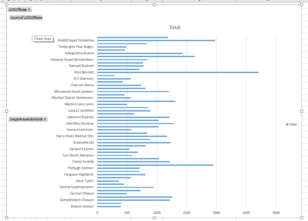
Now back in the pivot table, select the cell B4, right click, then choose Sort -> Sort Largest to Smallest.

Once that is done, you will see the chart updated as well. But now it is much easier to see what areas have the most crime – Ross Bennett is now at the top.

Next we are going to make it so our chart title will also update. Select the Total title area for the top of the chart. Then place the focus in the function bar area. Then select the cell B1. Once that is done, hit Enter.

Now go ahead and in the UCROffense filter, select Burglary-Business, and see what happens to the chart. Pretty cool eh!

Next we are going to place the chart in its own sheet. Select the chart area, then right click -> Move Chart…

In the pop-up dialog, select the New sheet option, and then name the sheet something more informative than Chart1, I named mine here UCR Offenses Slicer by TAAG.

And now you will see the chart is in its own worksheet. Now to make the chart alittle nicer. Go ahead and select the Total legend on the right hand side and delete it. Then in the PivotChart Fields area on the right select the TargetAreaActionGrids field, and select the Hide Axis Field Buttons option.

Do the same for the Count of UCROffense field as well. Now we only have the slicer for the UCR offense on our chart. You can go ahead and play around with this to check out other crime counts in areas. For nice images in reports please take out those buttons!

The last thing we are going to do is to filter this so we are only looking at the top 10 areas. Currently there are too many areas to even see label all of them on our chart. Go back to the worksheet that our pivot table is in. Then select the Top 10 option.

In the pop-up dialog, change it to Top 5, and then select OK.

My table keeps the ties, so here I actually have 6 areas listed.

If we go back to our chart now, it also is just limited to the Top 5 areas, since it is linked to the pivot table. Here I also increased the font size of the TAAG area names. But now we are golden.

For your homework, I want you to do two things:
HOUR function. Then you may need to refresh the pivot table data in the Analyze tab (available when editing a pivot table) to get that new column to show up.)Insert both of these into a Powerpoint presentation (for slicer chart just pick one crime and then include that graph as a picture), then export to PDF and turn that PDF homework in. Remember to make the tables and graphs look nice for the homework.